Necessary Modifications to the Strap-Down Inertial Navigation System Model for Non-Earth-Based Users
Tamer Mekky Ahmed
Head of Spacecraft Dynamics and Control Department, Space Division, National Authority for Remote Sensing and Space Sciences, Cairo, Egypt.
*Corresponding Author
Tamer Mekky AH,
Head of spacecraft dynamics and control department, Space Division,
National Authority for Remote Sensing and Space Sciences, 23 Joseph
Broz Teto Street, El Nozha El Gedida, Behind Cairo Airport, Cairo,
Egypt.
Tel: 00201117154201
Email: tamermekky@hotmail.com
Article Type: Research Article
Received: November 10, 2014; Accepted: November 17, 2014; Published: December 18, 2014
Citation: Tamer Mekky Ahmed (2014) Necessary Modifications to the Strap-Down Inertial Navigation System Model for Non-Earth-Based Users. Int J Aeronautics Aerospace Res. 1(2), 11-20. doi: dx.doi.org/10.19070/2470-4415-140002
Copyright: Tamer Mekky Ahmed © 2014 This is an open-access article distributed under the terms of the Creative Commons Attribution License, which permits unrestricted use, distribution and reproduction in any medium, provided the original author and source are credited.
Abstract
Strap-down inertial navigation system (SDINS) is considered as a highly sophisticated dead reckoning system. The SDINS consists mainly of two triads the first is the three gyros triad, and the second is the three accelerometers triad. Modeling the SDINS has achieved a lot of importance in the literature, especially for surveying applications. However, using the SDINS for spacecraft applications imply some modifications to the SDINS deterministic models used for surveying applications. Traditional models of the SDINS include the effect of the earth rotational rate on the SDINS instruments (gyros, and accelerometers). This effect must be removed from the instrument model if the SDINS is to be used onboard of a spacecraft simply because the spacecraft doesn’t rest on the earth, and thus doesn’t sense the earth’s rotational rate. Necessary modifications of the accompanying algorithms are derived analytically in the research at hand.
2.Acceleration Measurement
3.Commonly used Reference Frames
4.Theoretical measurements of a moving gyro triad
5.Modeling the INS
5.1.Mathematical notations
5.2.Time derivative of the rotation matrix
5.3.Calculation of position and velocity derivatives
5.3.1.Mechanization of inertial frame
5.3.2.Mechanization of earth centered fixed frame
5.3.3.Mechanization of navigation frame
5.4.Mechanization equations for land based users
5.4.1.Quaternion attitude representation
6.Attitude mechanization equations in terms of quaternion
6.1.Position mechanization equation
6.2.Attitude mechanization equations
7.Modification of the mechanization equations for space based users
7.1.Velocity mechanization equation
7.2.Attitude mechanization equations
8.Conclusion
9.References
Keywords
Strap-Down; INS; Accelerometer; Gyro.
Acceleration Measurement
Different researches and text books had discussed the inertial navigation system, or some of its components such as [1-4]. The inertial navigation system accelerometer consists of a proof mass m suspended from a case by a pair of springs, as illustrated in Figure. 1. Referring to Figure. 1, the input axis is indicated by the arrow. If the body to which the system is attached is accelerating along this axis by an acceleration, a, the proof mass will be displaced from its equilibrium position by an amount, x. From Newton’s law, the force affecting on the proof mass is equal to the mass times the acceleration. And from Hook’s law, the force generated by the springs are equal to the equivalent spring constant, K, times the displacement x. Thus, from Newton’s law we find that
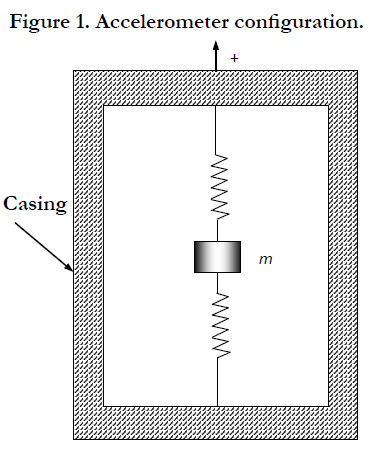
Fig. 1 Accelerometer configuration.
F = m a = K x ------(1)
Therefore the measured acceleration is
a = (K/m) x ------(2)
Consequently, acceleration in the plus direction causes the proof mass to move downward indicating positive acceleration. The displacement x is sensed using a pick-off and scaled to provide the value of acceleration. The proof mass equilibrium position is calibrated for zero acceleration. If the accelerometer is set on a bench in the earth’s environment, the gravity force will shift the proof mass downward w.r.t the case indicating positive acceleration. However, the gravitational acceleration is downward. For this reason, equation( 1 ) becomes
F = m (a-g) = K x ------(3)
And the measured acceleration is
a-g = (K/m) x = f ------(4)
Where, f is the specific force.
Commonly used Reference Frames
The earth centered earth fixed (ECEF) coordinates are defined such that the XE axis points towards the intersection between the Greenwich meridian and the earth’s equatorial plane, this point has a longitude and latitude (0,0) deg respectively [5]. The ZE axis of the ECEF axis is the earth’s rotational axis about itself. The YE axis is chosen to complete the right hand rule system.
The local-level (navigation) frame is defined such that X axis (E) points toward the east, Y axis (N) points to the north, and the Z axis (UP) points in the direction from the earth center to the INS origin. The ECEF and the navigation frame are illustrated in Fig. 2. The Geocentric-Inertial system has its origin at the earth’s center. The fundamental plane is the equatorial plane. The positive Z axis points in the direction of the North Pole, the positive X axis points in the direction of the vernal equinox on the first day of spring, and the positive Y axis completes the right handed set of coordinates. It is important to keep in mind that the inertial coordinate system is nonrotating w.r.t the stars (except for precession of the equinoxes).
The angle between the vernal equinox unit vector and Greenwich meridian is called αg –the “Greenwich sidereal time.” What we need is a convenient way to calculate the angle αg for any date and time of day. If we knew what αg was on a particular day and time we could calculate αg for any future time since we know that in one day the earth turns through 1.0027379093 complete rotations on its axis.
Suppose we take the value of αg at 0h UT on 1 January of a particular year and call it αgo. If, in addition, we express time in decimal fractions of a day, we can convert a particular day and time into a single number of days which have been elapsed since our “time zero.” If we call this number D, then
αg = αgo + 1.0027379093 x 360ox D [In Degrees]------(5)
or
αg = αgo + 1.0027379093 x 2π x D [In Radians]------(6)
Where
αgo = 1.74933340 rad at 1/1/1970 0h:0m:0s.------(7)
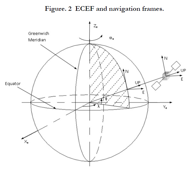
Figure. 2 ECEF and navigation frames.
The transformation matrix from inertial to ECEF coordinates is now computed from, The body system of axes is defined in Figure. 4.
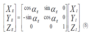
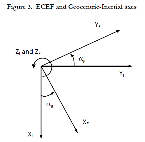
Figure. 3 ECEF and Geocentric-Inertial axes.
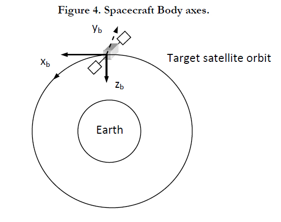
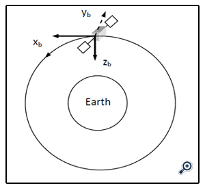
Figure. 4. Spacecraft Body axes.
Theoretical measurements of a moving gyro triad
The actual measurements of the accelerometers are the sum of the nominal measurements and the errors. If the accelerometers are stationary and miss-leveled by r, p, and θ errors about the x, y, and z body axes, they will measure a part of the gravitational force according to the relation.
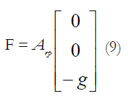
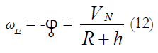
Where, Arpθ is the miss-alignment matrix. The nominal terrestrial usage of the gyros involves sensing the earth rotational components. As illustrated in Figure. 5, it is evident that the relation between the east velocity component and the longitude could be expressed as
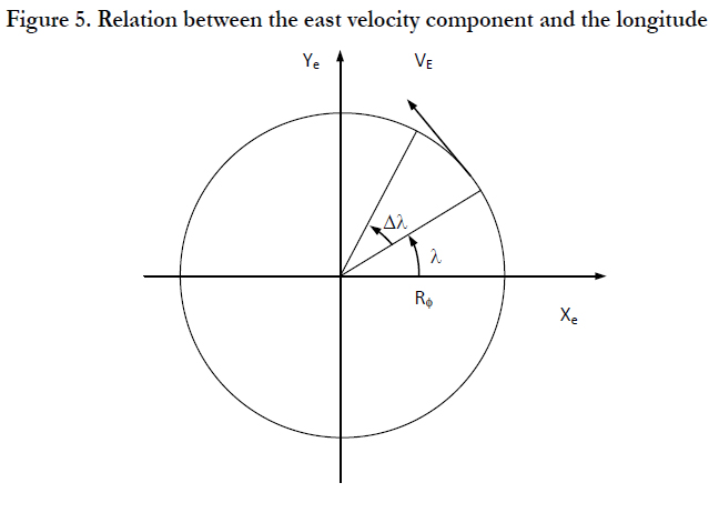
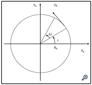
Figure. 5. Relation between the east velocity component and the longitude.
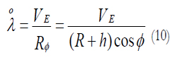
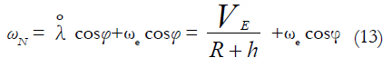
Referring to Fig. 6, we could also write
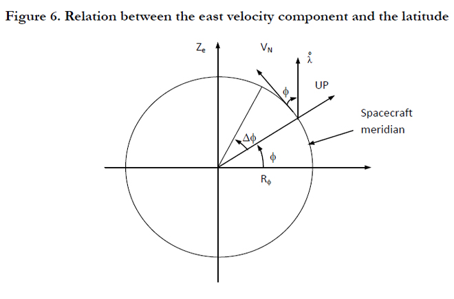
Figure. 6. Relation between the east velocity component and the latitude.
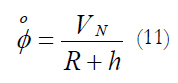
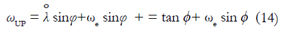
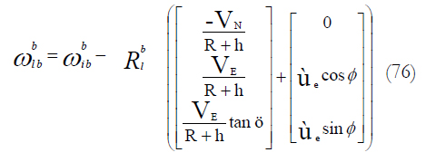
Where h is the spacecraft height. Finally, the local-level frame angular velocity components are
In this treatment we have assumed that the body frame and the inertial frame are aligned together. The relationship between the navigation frame and the INS body frame is usually established through either a stationary alignment process, or by continuous external velocity information from GPS receiver. Thus, the attitude angles are used in generating the rotation between the b-frame and the navigation frame. The rotation rates measured by the gyros are used to constantly update the transformation matrix between the body frame and the navigation frame. This transformation is used to transform the measured acceleration from the body frame to the navigation frame (in the case of strap down INS). Once transformed, integrating the acceleration twice will provide the INS position difference w.r.t. an initial point. However, as mentioned before, accelerometer measurements include both the platform and gravity, and hence knowledge of the gravitational field is mandatory to determine the platform acceleration. It is obvious that the INS is fundamentally dependent on an accurate knowledge of the initial position, velocity, and attitude of the moving platform prior to the start of INS operation.
The spacecraft center of mass position is given by re = [xe ye ze]T. Transformation matrices are used to transform any navigation vector from one computational frame to another. As an example, the position vector in the e-frame (earth fixed frame), re, is transformed to the i-frame (inertial frame) to give ri through the transformation matrix Rie, and hence
ri = Rie, re------(15)
Transformation from the i-frame to the e-frame is established throughout the inverse transformation, Therefore,
re=(Rie)-1 ri= Rie ri------(16)
And the angular velocity of the e frame w.r.t. the i frame is denoted as ωie . If this angular velocity is expressed in the e-frame, it will be denoted ωiee . The rotation between two coordinate frames can be expressed as a sum of rotations between different coordinate frames as
ωiee=ωile+ωlee------(17)
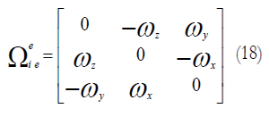
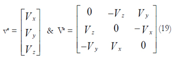
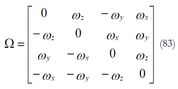
Rotation can be represented in two ways, an angular velocity vector, and a skew symmetric matrix comprising the same vector components. For example, the angular velocity vector ωiee may be represented either in a vector form ωiee = [ ωx ωy ωz]T, or in the skew matrix form
Similarly, the velocity vector could be expressed as
It is also important to note that coordinate transformations apply also to angular velocity vectors. As an example, the angular velocity vector, , could be transformed to the inertial frame using the relation
ωiee=Rieωiee-----(20)
The equivalent transformation between two skew-symmetric matrices has the special form
Ωiie = Rie Ωiie Rei------(21)
If we have two vectors a and b, their cross product a b can be expressed in terms of their skew symmetric matrices ( A or B) as
a x b = A b = -Ba -----(22)
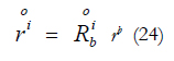
For a fixed point in a certain coordinate frame (body-frame) the position vector (r) can be transformed from the body frame, b, to the inertial frame, i, by the transformation
ri = Rib rb------(23)
Differentiation of both sides of equation ( 23 ) assuming that rb is constant (i.e. the point in spacecraft body is assumed to have a pure rotational motion without any translation) will give
The velocity of the body could be computed in the inertial frame from
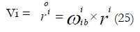
Using equation ( 22 )we could write equation ( 25 ) in the form
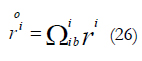
Substitution using equation ( 21 ), into equation ( 26 ) gives
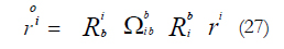
From equation ( 23 ) we could write equation ( 27 ) in the form
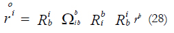
Since the matrix Rbi is the inverse of the Rib matrix, then RbiRib =I and equation ( 28 ) is reduced to
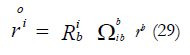
Comparing equation ( 24 ) with equation ( 29 ) we could easily deduce that
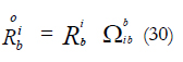
The vector ra is transformed from the a coordinate frame to the b coordinate frame according to the relation
rb = Rb + Rba ra------(31)
Where: Rb is the vector directed from the b-frame origin to the a-frame origin, and Rba is the matrix that transforms from the a-frame to the b-frame. If the a-frame rotates w.r.t. the b-frame, then differentiation of equation ( 31 ) gives
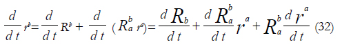
Substitution using equation ( 30 ), by replacing the subscript b with a and the super script i with b into equation ( 32 ) gives
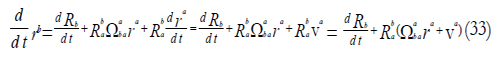
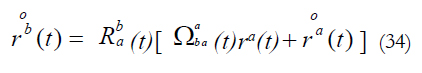
Equation ( 33 ) has the form of the coriolis theorem which states that, If two coinciding frames of reference experience relative angular rotation Ωaba(t) with rb(t)= Rbara(t), and Rba = RbaΩaba(t), then the time rate of change of the two coordinate systems are related by
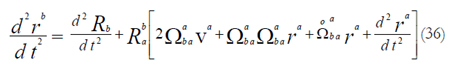
Taking the second derivative of equation ( 33 ) gives
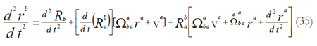
Substitution using equation ( 30 ) into equation ( 35 ) results in
place formula
From which we could write
The inertial body velocity can be expressed using coriolis equation using the following relation
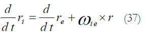
Differentiating equation ( 37 ) and letting d/dt re= ve, we get
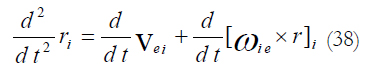
Application of equation ( 37 ) to the second term in the right hand side of equation ( 38 ) gives
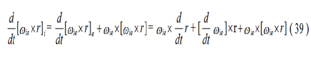
But the earth turn rate is constant, therefore [d/dt]=0, and equation ( 39 ) becomes
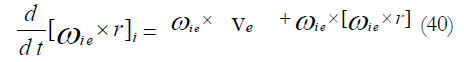
Equation ( 40 ) could now be substituted instead of the second term of equation ( 38 ) and this substitution results in
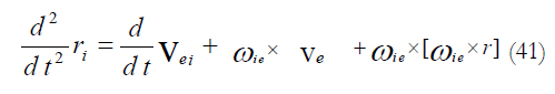
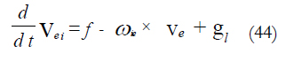
From which it is evident that
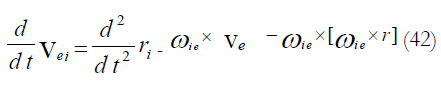
Equation ( 4 ) says that a = f + g, where a = d2/dt2 ri. Consequently, equation (42 ) becomes
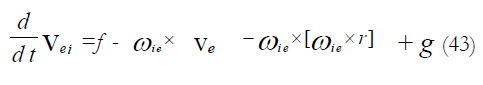
Looking carefully into equation (43 ) we could easily see that:
1-f : Is the specific force acceleration to which the INS is subjected.
2-ωie x ve : Is the coriolis acceleration.
3-ωie x [ωie x r]: Is the centripetal acceleration caused by the earth rotation with respect to an inertial frame.
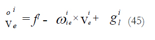
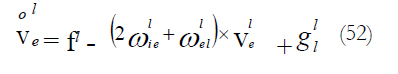
4-ωie x [ωie x r] + g : is the centrifugal acceleration representing the local gravity vector, gl. So equation (43) could be written as
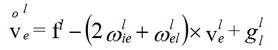
This equation could be expressed in the inertial frame of reference as
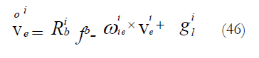
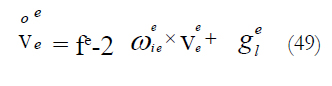
Using Coriolis equation, the ground velocity expressed in ECEF coordinate system, Vee , is differentiated with respect to time to give
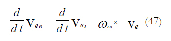
Substitution from equation ( 45 ) results in
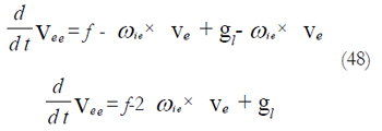
Expressing equation ( 48 ) in the ECEF axes gives
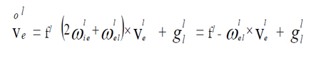
Mechanization of the navigation (local level) frame proceeds as the earth centered fixed frame mechanization. The derivatives of the ground velocity in the (local level) frame and the inertial frame of references are related by
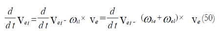
Substitution from equation ( 45 ) into equation ( 50 ) gives
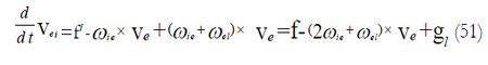
Equation ( 51 ) is expressed in the local level frame by
Referring to Figure.6, The earth rotation angular velocity vector is in the same direction of λ° , Thus for earth based users equations ( 12 ), ( 13 ), and ( 14 ) include the components of the earth’s angular velocity vector. As a result, let’s define
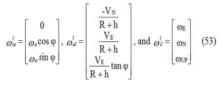
So equations ( 12 ), ( 13 ), and ( 14 ) could be put in the form
ωill=ωiel+ωell-----(54)
The first important note is related to the attitude mechanization equation. Applying equation ( 30 ) in the local level navigation frame results in:
Rl0b= Rlb Ωibb-----------------------(55)
But we know that
Ωlbb=Ωlib+Ωibb=-Ωilb+Ωibb=Ωibb-Ωilb------(56)
And
Ωilb=Ωieb+Ωelb-----(57)
Substitution from equation ( 57 ) into equation ( 56 ) gives
Ωlbb=Ωibb-(Ωebb+-Ωelb)------(58)
Consequently the attitude mechanization equations become
Rl0b= (Ωibb-Ωebb- Ωelb)------(59)
Where the Ωibb matrix is obtained from gyro measurements, Ωelb is the skew symmetric matrix corresponding to the vector Ωelb which could be obtained from
And similarly we could compute the skew symmetric matrix Ωieb from the corresponding angular velocity Ωieb vector which could be computed from
And Rib is the transformation matrix from the local level to the body frame defined by
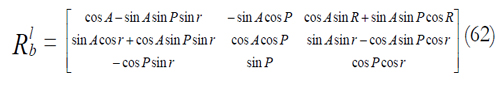
With P, the pitch angle (inclination), r is the roll angle, A is the azimuth angle.
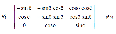
Finally, the transformation matrix from the local level to the earth fixed frame is given by
Quaternion parameters are introduced to describe the rotation of the b-frame w.r.t. the local level frame. The transformation matrix that transforms a vector from the reference frame to the body frame is a proper real orthogonal one. This means that it preserves the lengths of vectors and the angles between them, and also the inverse of the matrix is simply its transpose. So if A is the transformation matrix that transforms a vector from the reference to the body coordinate system, its transpose AT will transform that vector back to the reference system.
It is also known that a proper real orthogonal 3x3 matrix has at least one eigenvector with eigenvalue unity [7] and hence there exists a unit vector, ê that isn’t changed by A so that
Aê=ê------(64)
Which means that the vector ê has the same components along both body and reference axes, so ê is the axis of rotation. This demonstrates Euler’s theorem: “the most general displacement of a rigid body with one point fixed is a rotation about some axis”.
Referring to the transformation matrices described earlier, for a single rotation about single axis, we find that: for a rotation with single angle Φ the trace (sum of all diagonal elements) of the corresponding transformation matrix is
tr (A(ɸ))=1 + 2 cos ɸ------(65)
Generalizing this rule for any sequence of rotations, we may transform any successive rotations to a single rotation by an angle Φ about a unit vector (axis of rotation) such that
cosΦ= ½ [tr(A) -1]------(66)
Examining this equation, we find that it has two solutions for the Euler axis / angle Φ, which differ in sign only. The two solutions have the rotation axis vectors ê in opposite directions.
This means that a rotation about the vector ê by an angle Φ is equivalent to a rotation about the vector -ê by -Φ.
The Euler symmetric parameters are defined in terms of Euler axis / angle and the components of the axis of rotation ê as follows
q1 = e1 sin (Φ/2 )------(67-a)
q2 = e2 sin (Φ/2 )------(67-b)
q3 = e3 sin (Φ/2 )------(67-c)
q4 = cos (Φ/2 ) ------(67-d)
The four Euler symmetric parameters satisfy also the constraint
q21 + q22 + q23 + q24 = 1------(68)
The four parameters could be regarded as the components of a quaternion vector,
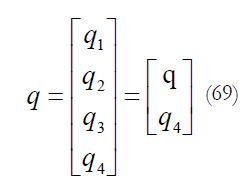
The direction cosine matrix could be expressed in terms of quaternion as in equation (70).
And also we could inversely express Euler symmetric parameters in terms of the direction cosine matrix as follows
q1 = ±0.5 (1+ A11- A22 - A33)½------(71-a)
q2 = ±0.5 (1- A11+ A22 - A33)½------(71-b)
q3 = ±0.5 (1- A11- A22 + A33)½------(71-c)
q4 = ±0.5 (1+ A11+ A22 + A33)½------(71-d)
Attitude mechanization equations in terms of quaternion
Based on the pre-discussed principals we could write
ωibb=ωilb+ωlbb------(72)
Where ωibb is sensed by the gyroscopes. Thus,
ωlbb=ωibb+ωilb------(73)
And similarly,
ωilb=ωieb+ωelb------(74)
we know that, ωieb=Rblωiel and ωelb=Rblωell . Thus we could write equation (74) as
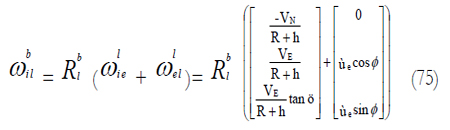
Substitution from equation (75) into equation (73) gives
In order to combine the parameters for two individual rotations we find that
[A(q'') ] = [A(q')][A(q) ]------(77)
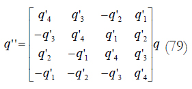
The resulting quaternion q" could be found from the final attitude matrix, or it could be in another different way [7]. If q" represents the orientation of the body frame with respect to the reference frame at time t + Δt ,q represents it at time t then represents the orientation of the body frame relative to the position that it occupied at time t, thus we could write
q'1=eu sin (Δø/2)------(78-a)
q'2=ev sin (Δø/2)------(78-b)
q'3=ew sin (Δø/2)------(78-c)
q'v=cos(Δø/2)------(78-d)
Where eu, ev and ew are the components of the rotation axis unit vector (i.e. they are in the direction of p, q and r), ΔΦ = ωΔt =√p2+q2+r2 Δt (this is valid only for an infinitesimal time interval Δt), also we may write
q"=qq'
Or in a matrix form
Replacing q' by the change in Euler axis/angle
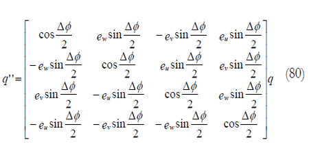
Thus we may possibly write
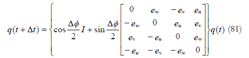
Where I is the fourth order identity matrix. In addition, all the right hand side terms are evaluated at time t. The former equation is mostly useful if the axis of rotation doesn’t change over the time interval Δt. For the case of attitude dynamics and prediction, equation (81) may be converted to a differential equation, though it may be used as it is to reduce the integration effort. Also small angles approximation will be used with the assumption of infinitesimal time period Δt to get
cos (ΔΦ/2) ≈1 and sin (ΔΦ/2) ≈ (ΔΦ/2) ≈ (ωΔt/2)
Noting that ω=ω ê=[ωx ωy ωz]T is the instantaneous angular velocity vector Finally we could write
q(t+Δt) ≈ [ID + Ω (Δt/2)]q(t)------(82)
And Ω is the skew-symmetric matrix
Where ωx, ωy, and ωz are the components of the angular velocity vector ωblb.
To go over the main points, the INS mechanization equations for land based users are summarized as
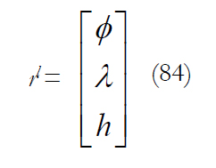
The position of a moving platform described in the l-frame is expressed in terms of the curvilinear coordinates (Φ,λ,h), where Φ is the latitude, λ is the longitude, h is the altitude. Thus, we could write
And from equations (10) and (11) we could write
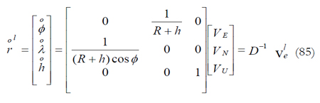
Using equation (52), we could write
Thus,
Equation (86) implies the existence of a gravity model. To simplify the problem, we present the simplest possible gravity model defined by [6]
g(h) = g(0) / (1+h/R)2------(87)
Where, g(0) = 9.780318 m/s2, and g(h) is the magnitude of earth gravitational vector defined in the local level frame by g = [0 0 –g(h)]T. The local gravity vector is thus
gll = g-ωie x[ωie x r]------(88)
The mechanization equations of attitude are given in equation (59) as R°lb = ( Ωbib-Ωbie-Ωbel ) or alternatively in equation (82) as q(t + Δt)≈[ID +Ω(Δt/2)]q(t), and Ωblb is given by its corresponding form of ωblb given by equation (76).
Modification of the mechanization equations for space based users
Looking carefully into equations (52), (53), and (54) we could deduce some important notes. First, the term ωlie, represents a component of the earth’s rotation sensed by a stationary INS (i.e. VE = VN = VUP = 0 m/sec) on the earth’s surface. For space based users, this term won’t be sensed by the INS at all. So, ωlie =0, and ωlil = ωlel. The second important note is related to the attitude mechanization equation. Applying equation (30) in the local level navigation frame results in:
Rl0b= Rlb Ωibb------(89)
But we know that
Ωblb=Ωbli+Ωbib=-Ωbil+Ωbib=Ωbib-Ωbil------(90)
And
Ωbil=Ωbie+Ωbel------(91)
Substitution from equation (91) into equation (90) gives
Ωblb=Ωbib-(Ωbie+Ωbel)------(92)
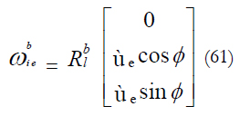
But Ωbie is the skew-symmetric matrix corresponding to ωbie which is equal to Rbl, and we also know that ωlie =0. Thus, equation (92) reduces to
Ωblb=Ωbib-Ωbel------(93)
Consequently the attitude mechanization equations become
Rlob = Rlb(Ωbib-Ωbel)------(94)
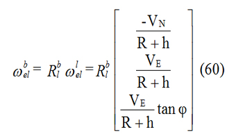
Where the Ωbib matrix is obtained from gyro measurements, Ωbel is the skew symmetric matrix corresponding to the vector ωbel which could be obtained from
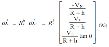
Using equation (52) in addition to that, ωlie=0 , we could write
Thus,
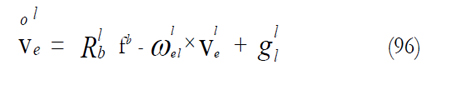
The gravity model given by equation (88) should now be modified to reflect the absence of earth rotation sensing by the accelerometers ( recalling that ωlie =0). So the gravity model becomes
gll = g −ωie × [ωie × r ]= g------(97)
The mechanization equations of attitude are given in equation (94) as Rlb= Rlb(Ωbib-Ωbel) or alternatively in equation (1.99) as q(t + Δt)≈[ID + Ωblb(Δt / 2) ]q(t), and Ωblb is now given by equation (93) instead of its corresponding form of Ωblb given by equation (76).
Conclusion
The most important conclusion coming out from this research is that the application through which the SDINS is used affects the associated mechanization equations and the gravity model. For terrestrial applications, the SDINS model is developed clearly with the appropriate systems of axes. If the SDINS is utilized by a user who isn’t resting on the earth the SDINS model must be modified according to section (7).
References
- Habib, T.,” New AlgorithmS of Nonlinear Spacecraft Attitude Control via Attitude, Angular Velocity, and Orbit Estimation Based on the Earth’s Magnetic Field”, PhD thesis, Aerospace Department, Cairo University, 2009
- Sumit, J., et al,” Preliminary Design of Solar Powered Unmanned Aerial Vehicle”, Applied Mechanics and Materials, Vol.225, Issue 1, 2012, pp. 315-322
- Jashnani, S., et al,” Sizing and preliminary hardware testing of solar powered UAV”, The Egyptian Journal of Remote Sensing and Space Sciences, Vol.16, 2013, pp. 189-198.
- Liu, X., et al,” A Method for SINS Alignment with Large Initial Misalignment Angles Based on Kalman Filter with Parameters Resetting”, Mathematical Problems in Engineering, Vol.2014, dx.doi.org/10.1155/2014/346291.
- Habib, T.,” The Global Positioning System Application to Satellite Position and Attitude determination”, MSc thesis, Aerospace Department, Cairo University, 2003.
- Shearman, and Bradsell, P.,” Strap-down Inertial Navigation Technology”, Peter Peregrinus Ltd., 1997.
- Wertz, J. R., “Spacecraft Attitude Determination and Control”, D. Reidel Publishing Company, 1997.