Commercial Cameras Accurate Focal Length Estimation for Satellite Optical Observation
Tamer M Ahmed1*, Karim K Ahmed2, Ayman H Kassem3
1 Researcher, National Authority for Remote Sensing and Space Sciences, Space Division, Spacecraft Dynamics and Control Department, Cairo, Egypt.
2 Engineer, National Authority for Remote Sensing and Space Sciences, Egyptian Space Program, Cairo, Egypt.
3 Professor of Automatic Control, Cairo University, Faculty of Engineering, Aerospace Department, Cairo, Egypt.
*Corresponding Author
Tamer Mekky Ahmed,
Researcher, National Authority for Remote Sensing and Space Sciences,
Space Division, Spacecraft Dynamics and Control Department, Cairo,
Egypt.
Tel/Fax: 00201117154301
E-mail: tamermekky@hotmail.com
Received: May 29, 2015; Accepted: August 06, 2015; Published: August 11, 2015
Citation: Tamer M Ahmed, Karim K Ahmed, Ayman H Kassem (2015) Commercial Cameras Accurate Focal Length Estimation for Satellite Optical Observation. Int J Aeronautics Aerospace Res. 2(4), 49-57. doi: dx.doi.org/10.19070/2470-4415-150006
Copyright: Tamer M Ahmed© 2015 This is an open-access article distributed under the terms of the Creative Commons Attribution License, which permits unrestricted use, distribution and reproduction in any medium, provided the original author and source are credited.
Abstract
Spacecraft orbit estimation based on optical observations captured by a commercial camera is considered to be a challenge. Camera focal length turned out to be a parameter of utmost importance. The main goal of this work is to develop different algorithms able to estimate the focal length of a commercial camera based on actual measurements (observations). Thirteen different algorithms, including different Kalman Filters, Genetic Algorithms, and Simulated Annealing, and three different cameras are used in this study. The results of these algorithms are compared in order to measure their efficiency and determine the best way to compute the focal length. It is found that the best performance (in terms of the selected cost function) is achieved by genetic algorithms. Estimation algorithms such as Kalman filters are useful when there is a large ambiguity associated with the value of camera focal length. The graphical solution is characterized by simplicity and relatively good performance.
2.Introduction
3 Process and Measurement Model
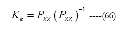
4.The Kalman Filter
5.Unscented Kalman filter (USKF)
4.Derivative free Implementation of the Extended Kalman filter
6.Filter Covariance
7.Observability Analysis
8.Finding the Global Optimum Solutions and Formulation of the Cost Function
9.Experimental validation
9.1.Estimation algorithms
9.2.Iteration based methods
10.Conclusion
11.References
Keywords
Commercial Camera; Optical Observation; Estimation Algorithms; Genetic Algorithms; Simulated Annealing.
Introduction
Commercial camera utilization for space applications has attracted the attention of vast number of researches. Accurate spacecraft attitude determination requires a good estimation of the camera optical parameters. For star sensors, it is common to estimate focal length, optical distortion, and principal point. These parameters are considered to be critical for star identification algorithms which are utilized to identify certain stars located at the captured image. This process is usually characterized by a huge computational effort which is very sensitive to these parameters. Samaan M (2012) utilizes a commercial off-the-shelf camera as a low cost star tracker. Camera optical parameters and lens distortion are estimated in Zhou F (2015), Dzamba T (2009), discusses the problem of characterization of field curvature and lens astigmatism aberrations. Pal M, Bhat M (2009), solves the problem of spacecraft attitude determination independent of the problem of camera calibration except for the distortion of the camera lens. The star spot location is estimated in Liu HB (2011) based on Kalman filter only. Samaan MA (2001) uses only two methods to estimate the camera focal length. Samaan MA (2003) used the least squares to optimally estimate the focal length.
Spacecraft in-orbit failure could be divided into, mechanical failure, software failure, electrical failure, and unknown [8]. When a spacecraft is totally lost due to any of these reasons, it is necessary to determine whether it is still in-orbit or not. If such a case is encountered, the optical observation of the spacecraft is an optimum choice to assure that the spacecraft is still in-orbit, see [9] for more details. In addition, optical observations could help to increase the accuracy of orbit predictions. Nowadays, commercial cameras could be used instead of complex, heavy, and expensive telescopes for optical observations. Spacecraft orbit estimation based on optical observations captured by a commercial camera is considered to be a challenge that has never been posed before. The nature of the process of spacecraft optical observation is somehow different than that of star identification. Thus, the critical parameters of the two processes are not the same. For, the problem of spacecraft optical observation the camera focal length is considered to be the main parameter of utmost importance.
The contribution of this research is to use approximately costless algorithms of commercial camera calibration for the purpose of spacecraft orbit determination. We should also take into account that the problem of spacecraft orbit estimation, based on optical observations captured by a commercial camera, is considered to be a challenge. Thirteen different algorithms are utilized such as Kalman filter, unscented Kalman filter, derivative free implementation of the extended Kalman filter, genetic algorithms,and simulated annealing are utilized to accurately determine the camera focal length based on actual measurements provided by the camera. The results of all of these algorithms are compared to each other in terms of an error cost function that needs to be minimized.
Process and Measurement Model
The camera focal length is commercially provided by its manufacturer. The utilized camera model in this research is supposed to have a minimum focal length of 4mm. The process model is given by
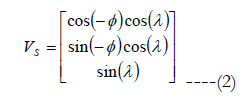
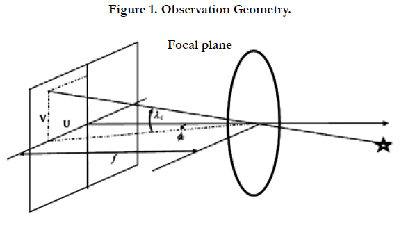
Figure 1. Observation Geometry.
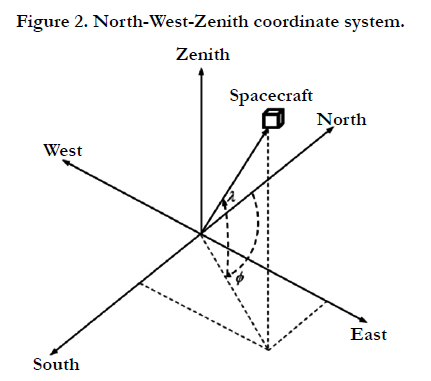
Figure 2. North-West-Zenith coordinate system.
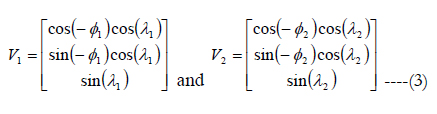
The first and the second star unit vector expressed in the North West Zenith (NWZ) system of axes is given as
U : Is the measured horizontal distance of a reference object imaged by the camera at the focal plane.
V : Is the vertical distance of a reference object imaged by the camera at the focal plane.
Φc : Object azimuth angle with respect to camera body axes.
λc : Object elevation angle with respect to camera body axes.
Thus, we have two sets of measurements.
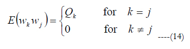
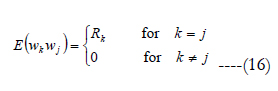
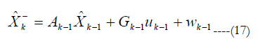
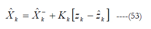
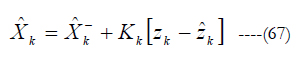
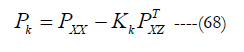
Traditionally, the Kalman filter was used to estimate system states and reduce the effect of noise and disturbances. The best estimate is chosen such that, the expected value of the error squares’ sum is minimum. So,
wk-1 : Is the process noise characterized by.
A k: State transition matrix.
Xˆk : Priori estimate of the state.
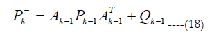
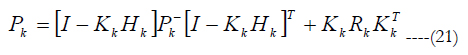
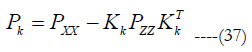
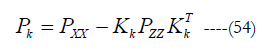
Pk : A posteriori covariance of the estimation error.
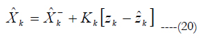
Xˆk : A posteriori state estimate.
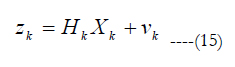
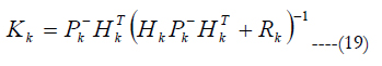
H k : Measurement matrix.
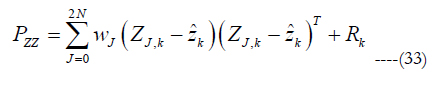
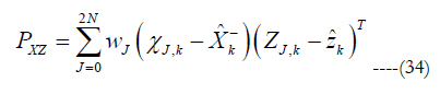
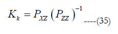
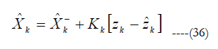
Unscented Kalman filter (USKF)
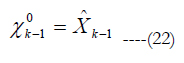
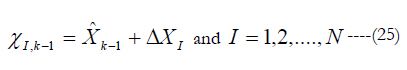
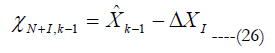
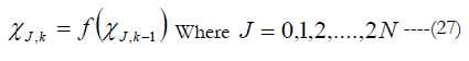
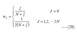
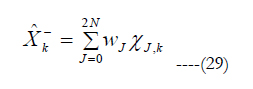
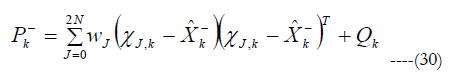
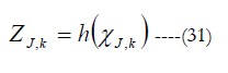
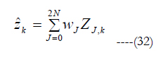
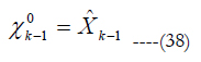
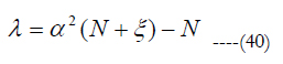
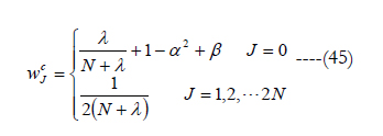
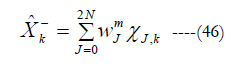
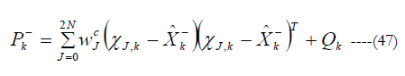
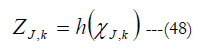
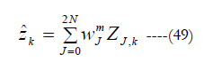
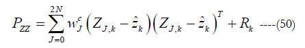
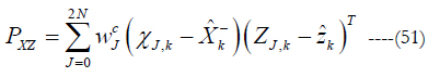
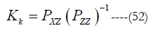
The unscented Kalman filter algorithm follows the fundamental steps of the Extended Kalman Filter (EKF). The difficulties associated with the traditional EKF are alleviated by the USKF. The filter basic structure given in [11], and [12] is briefly reviewed in this section. The USKF prediction stage starts by forming (2N+1) sigma points as follows
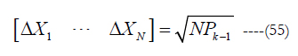
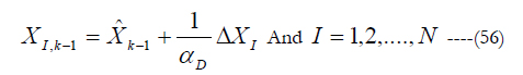
Derivative free Implementation of the Extended Kalman filter (DFEKF)
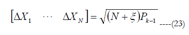
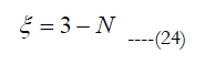
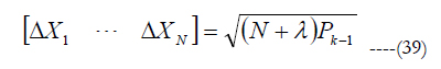
Derivative free implementation of the extended Kalman filter was firstly developed in [14]. If the number of filter states are given as N, then N vectors, ΔX1 , ΔX2, …. ΔXN, could be formed as follows,
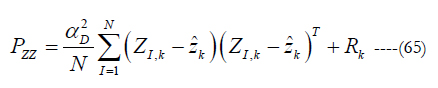
Filter Covariance
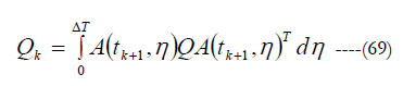
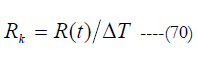
The process noise covariance, Q k, in its discrete form is related to its continuous form, Q , by the following equation [15]
Observability Analysis
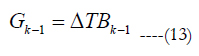
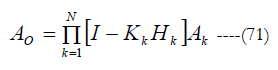
The filter state transition matrix based on Floquet theory for a discrete time system is given by [17]
Finding the Global Optimum Solutions and Formulation of the Cost Function
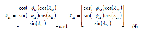
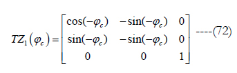
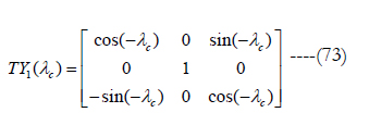
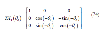
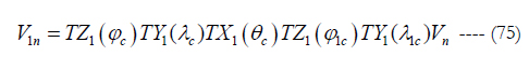
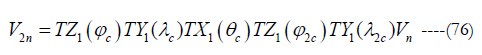
It is well known that there exists several algorithms to find global optimum solutions (i.e. finding the minimum or maximum) of a certain cost function. Genetic algorithms, and simulated annealing could be used efficiently for such purpose. These algorithms will not be reviewed herein. The reader should refer to standard text books such as [18] to find more relevant information. Camera attitude with respect to NWZ coordinate system is represented by three rotations φc , λc , θc around three independent axes, Z, Y, and X respectively. Thus, for the first star, we could write down the following transformation matrices
Experimental validation
The performance of the prescribed estimation algorithms is evaluated based on actual measurements. The estimation error is plotted in Figure.1 for the three algorithms which are namely: the Kalman filter (KF), the derivative free Kalman filter (DFEKF), and the unscented Kalman filter (USKF). The error is measured with respect to a simulated camera that has a focal length equal to that was given at the obtained image prosperities written by the camera for each image. Three camera models are used in this research, Benq GH600, Canon PowerShot SX150 IS, and Samsung DV100 Digital camera. Figure.3. Shows the estimated focal length using KF, DFEKF, USKF, in addition to the measured focal length based on λ measurements (LM) and Φ measurements (PM) respectively of the camera model Benq GH600. All of the calibration images have a theoretical focal length of 4mm as indicated by the prosperities of the images.
As clear in these figures the filters have succeeded in filtering the high noise associated with measurements. In addition, the estimator is able to converge quickly despite of large initial estimation error, which is thrown in purpose to prove the high performance of the estimator. The maximum Eigen values of A0 the matrix is 2.9×10-152 which is a very small value that indicates a high rate of convergence. If the measurements were smoothed, the resulting estimated focal length is shown in Figure 4.
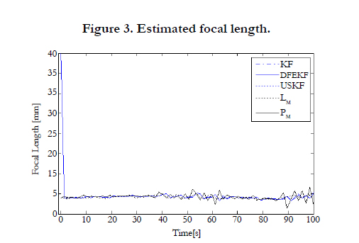
Figure 3. Estimated focal length.
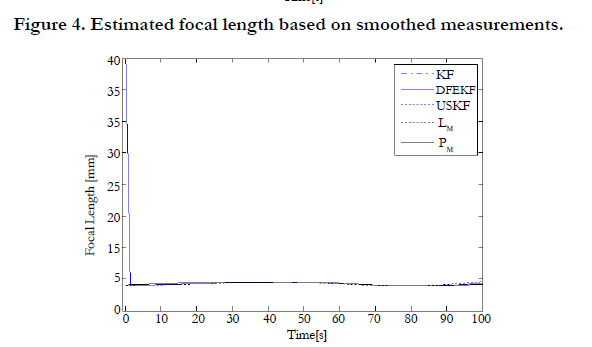
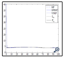
Figure 4. Estimated focal length based on smoothed measurements.
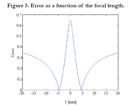
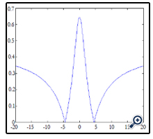
Figure 5. Error as a function of the focal length.
The required parameters to be determined from the image are camera attitude angles and focal length. The proposed algorithm scans a range of focal lengths, and for each foal length solves for the attitude angles using the triad method, and finally computes an error. At this point there are several algorithms are adopted as follows:
Algorithm A: The range of focal lengths is selected and scanned by the simply evaluating the error corresponding to each focal length, and the focal length with minimum error is chosen based on simple gridding technique.
Algorithm B: The error is plotted versus the focal length, and the focal length is selected graphically from the graph, as shown in Figure.5. As clear in this figure the error function is even.
Algorithm C: The focal length is determined based on genetic algorithms.
Algorithm D: The focal length is determined based on simulated annealing.
Algorithm E: The focal length and camera attitude are determined based on simple gridding.
Algorithm F: The focal length and camera attitude are determined based on genetic algorithms.
Algorithm G: The focal length and camera attitude are determined based on simulated annealing.
A comparison among all of the utilized algorithms is given in Table 1.
As shown in Table.1. The best performance (in terms of the selected cost function) is achieved by algorithms G, and F respectively. Algorithms A, B, C, D, E, and F show medium performance. Data smoothing has enabled estimation algorithms to enhance their performance. There are also some important otes those must be mentioned regarding estimation algorithms. The first note is that the cost function that is minimized by these estimation algorithms is given by equation (7) not equation (77). So, their performance is not the best in terms of the formed cost function defined in equation (7).
Therefore, these algorithms obtain lower performance in terms of the cost function defined by equation (77) than the other algorithms. The second note that should be mentioned is that these algorithms converge quickly, nearly in the second time step despite of large initial estimation error because of the strong observability indicated by the small Eigen values of equation (71). Consequently, it is considered to be a good design approach to initialize the process of focal length estimation based on estimation algorithms and then proceed to a fine tuning process by using iteration based algorithms such as algorithm F. On the other hand, estimation algorithms are complex and require lots of mathematical treatment. The simplicity of medium performance algorithms such as Algorithm B, may represent an advantage even though they are characterized by medium performance. The algorithms presented in Table 1 are applied for two camera models which are Canon PowerShot SX150 IS (Table 2), and Samsung DV100 (Table 3) Digital camera respectively. As clear in both tables, algorithms B, and F, usually achieve a very good performance. This result is identical to what is obtained in Table 1.
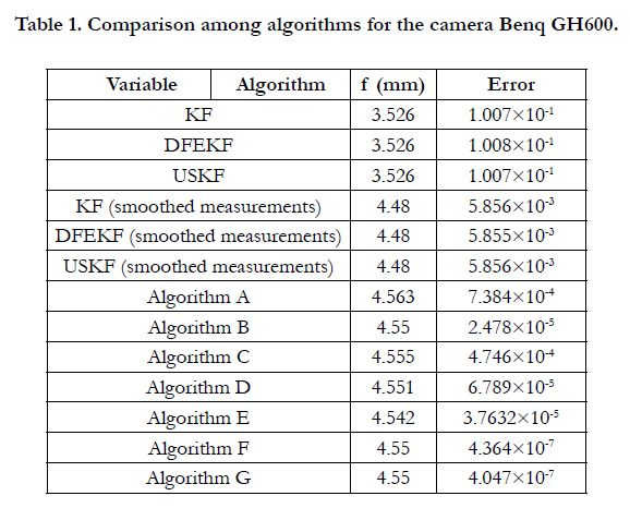

Table 1. Comparison among algorithms for the camera Benq GH600.
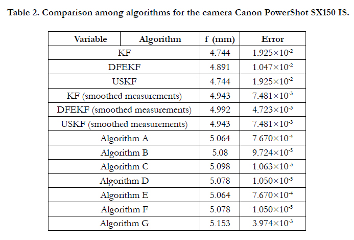
Table 2. Comparison among algorithms for the camera Canon PowerShot SX150 IS.
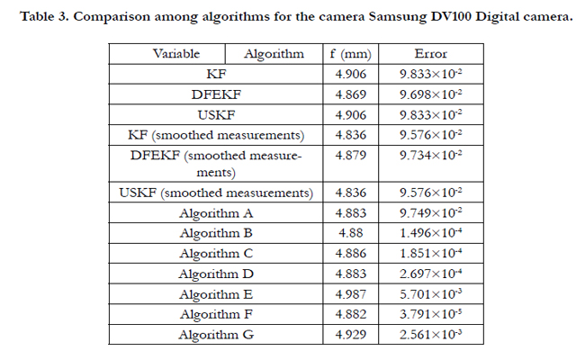
Table 3. Comparison among algorithms for the camera Samsung DV100 Digital camera.
Conclusion
The problem of camera focal length determination has turned out to be of much importance for the purpose of spacecraft orbit observation based on commercial camera instead of large, heavy, complex, and expensive telescopes. Thirteen different algorithms are examined extensively to solve this problem. A comparison among these algorithms showed that estimation algorithms are able to converge despite of large initial estimation error. The performances of these algorithms are enhanced if they are preceded by the process of measurement smoothing. On the other hand estimation algorithms are characterized by complexity and low performance in terms of the cost function defined by equation (77). Some medium performance algorithms such as Algorithm B are characterized by their simplicity compared to estimation algorithms. Algorithms G, and F, exhibit high performance but they are based on iteration. Accordingly, a good design approach could be achieved if estimation algorithms are used first, and then a fine tuning process is performed by using an iteration algorithm such as algorithm F.
References
- Samaan M, Theil S (2012) Development of a Low Cost Star Tracker for the SHEFEX Mission. Aerospace Science and Technology 23(1): 469-478.
- Zhou F, Ye T, Chai X, Wang X, Chen L (2015) Novel Autonomous On- Orbit Calibration Method for Star Sensors. Optics and Lasers in Engineering 67: 135-144.
- Dzamba T (2009) Calibration Techniques for Low-Cost Star Trackers. MSc thesis, Ryerson University, Toronto.
- Pal M, Bhat M (2009) Star Camera Calibration Combined with Independent Spacecraft Attitude Determination. American Control Conference 4836-4841.
- Liu HB, Yang JK, Wang JQ, Tan JC, Li XJ (2011) Star Spot Location Estimation Using Kalman Filter for Star Tracker. Applied Optics 50(12): 1735- 1744.
- Samaan MA, Griffith T, Singla P, Junkins JL (2001) Autonomous On-Orbit Calibration of Star Trackers. Core Technologies for Space Systems Conference. 1-18.
- Samaan MA (2003) Toward Faster and More Accurate Star Sensors Using Recursive Centroiding and Star Identification. PhD thesis, Texas A&M University. 1-134.
- Tafazoli M (2009) A Study of On-Orbit Spacecraft Failures. Acta Astronautica 64: 195-205.
- Habib TM (2014) Egyptsat; an Integrated Road Map for Suggested Research Points – Astrodynamics Perspective. ISNET/TUBITAK UZAY Workshop on Small Satellite Engineering and Design for OIC Countries.
- Wertz JR (1997) Spacecraft Attitude Determination and Control. D. Reidel Publishing Company, USA.
- Julier S (1997) Process Models for the Navigation of High-Speed Land Vehicles. PhD Thesis, Department of Engineering Science, University of Oxford, UK.
- Bhanderi D (2005) Spacecraft Attitude Determination with Earth Albedo Corrected Sun sensor Measurements. PhD Thesis, Department of Control Engineering, Aalborg University, Denmark.
- Roh K, Park S, Choi K (2007) Orbit Determination Using the Geomagnetic Field Measurement Via the Unscented Kalman Filter. Journal of Spacecraft and Rockets 44(1): 246-253.
- Quine B (2006) A Derivative-Free Implementation of the Extended Kalman Filter. Automatica 42(11): 1927-1934.
- Smyth A, Wu M (2007) Multi-rate Kalman filtering for the data fusion of displacement and acceleration response measurements in dynamic system monitoring. Mechanical Systems and Signal Processing 21(2): 706-723.
- Brown RG, Hwang PY (1997) Introduction to Random Signals and Applied Kalman Filtering. John Wiley and Sons, Inc., New York. 290-291.
- Psiaki M, Martel F, Pal P (1990) Three Axis Attitude Determination via Kalman Filtering of Magnetometer Data. Journal of Guidance, Control and Dynamics 13(3): 506-514.
- Jamshidi M, Coelho L, Krohling R, Fleming P (2002) Robust Control Systems with Genetic Algorithms. CRC Press, USA. 3: 232.
- Habib TM (2013) A Comparative Study of Spacecraft Attitude Determination and Estimation Algorithms (A cost-benefit approach). Aerospace Science and Technology 26(1): 211-215.