AI, Deep Machine Learning via Neuro-Fuzzy Models: Complexities of International Financial Economics of Crises
Haider A. Khan*
JKSIS, University of Denver, USA.
*Corresponding Author
Haider A. Khan,
JKSIS, University of Denver, USA.
Tel: 303-871-4461/720-748-2555
E-mail: hkhan@du.edu
Received: September 07, 2021; Accepted: November 11, 2021; Published: November 16, 2021
Citation:Haider A. Khan. AI, Deep Machine Learning via Neuro-Fuzzy Models: Complexities of International Financial Economics of Crises. Int J Comput Neural Eng. 2021;7(3):122-134. doi: dx.doi.org/10.19070/2572-7389-2100016
Copyright: Haider A. Khan© 2021. This is an open-access article distributed under the terms of the Creative Commons Attribution License, which permits unrestricted use, distribution and reproduction in any medium, provided the original author and source are credited.
Abstract
This paper addresses one of the five major areas of AI research identified by Domingos in computer science. I demonstrate
that certain Artificial Intelligence (AI) and Machine Learning (ML) type of modeling has great relevance for difficult areas of
financial economics and complex financial systems analysis. In a neural network and fuzzy set theoretic formal setting, the ML
model predicts the currency crises by combining the learning ability of neural networks and the inference mechanism of fuzzy
logic. The empirical results show that the proposed neuro fuzzy model can not only provide better prediction (for both insample
and out-of-sample data) but also model causally more detailed relationships among the variables through the obtained
knowledge base. Additionally, causal structural path analysis can have significant implications for policy making. The (partially
identified) causal path scan also be the bases for further theoretical modifications. One interesting feature of this approach is
that it points towards the salient causal role of deep inductive learning in the study of financial crises.
2.Review of Literature
3.Conclusion
4.References
Keywords
Learning Algorithms; Artificial Intelligence(AI); Deep Machine Learning (ML); Currency Crises; Neuro Fuzzy Model; Signal Aproach; Logit; Econometrics.
Introduction
A General Background of AI ResearchLeading to Specific Neuro-
Fuzzy Type of Machine Learning for Better Understanding
and Prediction of Financial Crises:
Since the pioneering work by some economists during the early
years of the 21st century, other economists have increasingly recognized
that they have good reasons to be interested in AI and
machine learning. For example, a paper by [20] makes an interesting
and highly relevant comparison between the language of
econometrics and the language of Artificial Intelligence(AI) and
Machine Learning.[20] “…discuss a list of tools that … should
be part of the empirical economists’ toolkit and that …should
be covered in the core econometrics graduate courses.”(p.3) They
cover a wide-ranging list of topics and point out usefully that the
nature of the economic problem should dictate the ML algorithmic
modeling that can be the most relevant. In particular, the
causal structure2 of the relevant economic model derived from
an appropriate theory should dictate what kind of ML model one
should use. I agree with this logic and try to follow it by presenting
a particular model of inductive learning that can be embedded in
a neuro-fuzzy learning model for predicting, among other things,
financial crises. Of course, financial crises are among the most
intractable areas of (financial) economics. The claim on behalf
of the neuro-fuzzymodel (NFM) ML algorithmic approach(from
now on NFM-ML approach) is not that it is absolutely the best
predictor with all causal pathways clearly identified once and for
all. Rather it is a relative and comparative claim. In keeping with
scientific realism, the claim here is that relative to and in comparison
with commonly used econometric models, this AI-derived
ML approach performs better, given the available data and the
cognitive model of inductive learning3.
As Domingos (2015) points out, the hope for researchers on what
he calls “master algorithm” is to find an algorithm that can perform all the given tasks of AI, with sufficient and relevant data on
which ML is to be trained . But he is careful to note the limits of
the so-called “Big Data” because ‘sufficient’ data means, in some
cases, that the data required for the model can be infinite. Learning
from finite data means making specific assumptions, which
may not be of use in all the cases. This is true of the class of all
P and NP-complete problems4. If we think of a Turing machine
for computational problems as a deductive procedure, the search
for AI algorithms can be conceived as the ever more intelligent
inductive search for algorithms that can use data efficiently. One
solution for such a problem is that the necessary assumptions
(with a few restrictions) can also be fed to the algorithm as an
explicit input along with the original input, thus granting the user
the flexibility of plugging the necessary attributes or even create
new ones.
The hypothesis of the Master Algorithm is:
‘All knowledge – past, present and future- can be derived from data by a
single, universal learning algorithm.’5
If such an algorithm is possible, inventing it would be one of the
greatest scientific achievements of all time. In fact, the Master Algorithm
(MA) is the last thing we will ever have to invent because,
once we let it loose, it will go on to invent everything else that can
be invented. All we need to do is provide it with enough of the
right kind of data, and it will discover the corresponding knowledge.
However, since the MA is not yet within reach, Domingos
suggests five main families that are collectively close to being an
MA. These five are:symbolists, connectionists, evolutionaries,
Bayesians and Analogizers, Each has its strengths and limitations.
In this paper I elucidate a more modest claim than being the top
claimant to MA. I show the relevance and efficacy of NFM-ML
for analyzing one subset of challenging problems in International
Financial Economics.
Of the five families, I would argue, NFM-ML has a great potential
for computational economics of complex financial systems.
I demonstrate this through a concrete NFM machine learning
exercise and carry out predictions that can be compared with
econometric models derived from statistical theory. This is the
procedure of causal comparison from the perspective of scientific
realism defended by Miller(1987) and Khan(2008; 2019).
The insight from neuroscience that has been used by researchers
in NFM-ML is that, even the human brain functions on the
basis of a variety of algorithms that seem to all belong to a parent
algorithm uncovered by recent research. For example, we can
cite the results of an experiment where the process of rewiring
the brain by swapping the respective nerves did not result as how
the researchers expected it to be as a severely dysfunctional animal.
Instead, the respective nerves learnt to do the other nerve’s
functions, i.e. when the visual input is redirected to the somatosensory
cortex, which is responsible for touch perception, it also
learns to see. This is the primary principle of the ‘echolocation’
procedure for the blind people by clicking their tongue and listening
to its echoes without bumping into obstacles. With the help
of such algorithms, the blind can even play some sports. All of
this is evidence that the brain uses the same learning algorithm
throughout, with the areas dedicated to the different senses distinguished
only by the different inputs they are connected to the
different organs of the body. Perhaps in the formation of the
cortex, the same wiring pattern with local variations is repeated
everywhere. The learning mechanism is also the same: memories
are formed by strengthening the connections between neurons
that fire together, using a biochemical process known as longterm
potentiation similar to the neurobiological concept called
clustering. The most important argument for the brain being the
“Master” Algorithm, however, is that it is responsible for everything
we can perceive and imagine. Most importantly, the brain
learns through layers of neural networks. This is essentially what
thetheorists who proposed ---for example---the backward propagation
mechanism with hidden layers in complex neural network
learning procedure used to model Hebbian learning in a detailed
way [85, 86].
In international finance, since the breakout of the 2008 advanced
countries’financial crisis, there have been much attention devoted
to the construction of the early warning systems. In fact, this
started with the Asian Currency and Financial Crises [62]. In fact,
the motivation came from the European currency crisis in 1992
and the Mexican currency crisis in 1994 preceded the Asian crisis
in 1997 which was followed by the Russian currency crisis in 1998.
But especially since 2008, the search for an effective early warning
system has become a particularly important issue.
There have been a lot of related research in macro and financial
economics since Krugman’s 1979 contribution. Using a broad
classification approach, these contributions can be divided into
four main categories. The first set of papers all emphasize the
qualitative dimensions, exploring the change of important indicators
before the crisis. However, these papers did not conduct
rigorous empirical testing using these indicators [36, 46, 70, 74]. A
second group of papers have emphasized the difference between
the variables during the crisis period and non crisis period [39, 43,
77]. Yet a third set of paper have stried to predict the probability
of the crisis according to some theoretical model for example
[25]. This set can also be subdivided into two further categories,
single country models [31, 56, 82] and multiple countries’ models
[29, 43, 68, 75], including some papers using macro economic
variables to explain the contagion-related phenomena as well [87].
Finally in our fourth category, some researchers like Kaminsky
and Reinhart (1996) propose the signal approach to construct the
early warning system. However, according to Chowdhry and Goyal
(2000), the forecasting results of the out-of-sample periods for
Asian crisis are disappointing for most of the theoretical models
that use the signal approach. The inference to draw from such
critiques is that this problem of building early warning system
for financial crisis still needs further investigation. The possibility
of non-linear causal relationship among the variables ordered according to a complex causal structure motivates this paper to
explore the problem via a particular AI-based machine learning
approach.
As far as the nonlinear learning problem is concerned, the progress
in artificial intelligence approach to learning in the 1980s
and afterwards---- starting with Hinton’s path breaking contribution
in 1986--- has provided an alternative methodology to make
steady advances towards a global solution to the signaling problem6.
As is already clear from practical experience, expert systems,
fuzzy logic, and neural network approach all have been of use to
the managers who have to make decisions. However, although
the standard expert system algorithm can embed the experience
into the system, it is often too rigid to learn effectively with flexibility.
The neural network---particularly after Hinton’s contributions---
can learn more flexibly from relevant historical data. Furthermore,
in neural networks with fuzzy logic an algorithm can
describe the problem in the way close to the human being’s reasoning
process and accommodate the inaccuracy and uncertainty
associated with the data from the real world or from experiments
with human subjects. It stands to reason that a method which
can combine the advantages of neural networks and fuzzy logic
can be a more flexible algorithmic approach to learning problems.
Therefore, following this line of thinking, I present a model that I
have constructed with some colleagues for learning in the uncertain
environment of the financial markets. It is a hybrid of neural
network and fuzzy logic with inductive machine learning capacity.
Here I present the specific example of an application in order to
construct a currency crisis early warning system. In addition to
providing better out-of-sample forecasting results, the proposed
model also aims to providing a knowledge base to describe the
complicated relationship among the variables. Such aknowledge
base can provide a more concrete way to predict in a boundedly
rational way or with some luck, even help prevent--- or at least
mitigate the effects of---an impending crisis. This paper is structured
as follows. Section 2 is the relevant literature review of the
early warning model construction efforts. The construction of
neuro fuzzy model and its benchmarks are described in section
3. Section 4 presents the broader research methodology. The empirical
results are shown and discussed in section 5.s Conclusionsand
a discussion offurther research problems follow in section 6.
Literature Review for early warning model construction
In terms of the early warning model construction, usually a multivariate
logit model or a multi-variate probit model is constructed
to predict the probability of the occurrence of the crisis for the
next period or the next k periods. Although the explanatory variables
are not exactly the same for most of the papers, the estimation
technique is quite consistent. On the other hand, an alternative
is to check the difference of the selected variables between
before the crisis and during the crisisto see which variables can
be helpful in predicting the crisis. Kaminsky and Reinhart (1996)
proposed the signal approach to construct a warning system by
modifying this method.
The advantage of logit or probit model is to represent all the
information contained in the variables by giving the probability
of the crisis. The disadvantage is that it cannot tell the forecasting
ability of each variable though it can give the significance level
of each variable. In other words, the ability of the correct signal
and false alarm for each variable cannot be seen from the model.
Therefore, it cannot provide the clues where the problem is and
how to improve it, which is not beneficial for the authority to
monitor and to prevent.
On the other hand, the signal approach proposed by Kaminsky
and Reinhart (1996) can show the contribution (the percentage of
correct signal and the percentage of false alarm) of each variable
for the crisis prediction. Besides, it can also construct a summary
indicator by calculating the conditional probability given the number
of indicators signalizing. Later on, there are some researchers
studying on the difference between this method (signal approach)
and log it. Berg and Pattillo(1999) tries to predict the currency
crisis in 1997 by using the signal approach based on the work of
Kaminsky Lizondo and Reinhart(1998), the probit model based
on the work of Frankel and Rose(1996), and the regression model
based on the work of Sachs Tornell and Velasco(1996). The empirical
results show that the performance of all these three methods
are not significant.
As for the explanatory variables, Kaminsky Lizondo and Reinhart(
1998) divide the variables into seven categories, external,
financial, real sector, fiscal, institutional/structural, political, and
contagion by summarizing from 105 indicators in 17 papers. Finally
15 variables are selected to construct the warning system by
using signal approach. This paper has done an excellent job to
explore the related leading indicators for the currency crisis.
From the empirical results of the above literature it can be seen
that the conclusions may be inconsistent due to the different
explanatory variables, different data frequency (monthly data or
quarterly data), and different models employed. Besides, some
variables are significant for single variable model but insignificant
for multi-variate model due to the possible multicollinearity. Most
of all, a theoretical model which can provide an effective outof-
sample prediction is still unavailable. Therefore, this paper is
trying to construct a warning model through a different approach
in the hope to not only provide a better out-of-sample prediction,
but also can provide a more detailed relationship among the variables,
which can be the basis for further modification of the existing
theory and can provide the financial authorities more effective
ways to prevent or mitigate a financial crisis.
This paper is different from the earlier literature in the following
manner:
First, it is a data driven method to extract the relationship among
the variables from the historical data. The obtained relationship
can be the reference for theoretical modification of the existing
theory. Second, it is an inter-disciplinary effort to use cognitive
science and artificial intelligence tools to understand the international
financial economics domain problem of the currency crisis.
This crisis had not been explored using such an approach until we
constructed the first such interdisciplinary model. Needless to say,
one advantage of the nero-fuzzy modeling approach is that it puts
in sharp relief the question of the forecasting accuracy for both
in-sample and out-of -sample data.
The Construction Of The Competitive Warning Models For Causal Comparison7
Signal Approach
The basic philosophy of this approach is that the economy behaves
differently on the eve of financial crises and that this aberrant
behavior has a recurrent systemic pattern. For example,
currency crises are usually preceded by an overvaluation of the
currency; banking crises tend to follow sharp declines in asset
prices. Let A and B represent the number of times signaling
when there is really a crisis to happen and no crisis to happen
in 24 months respectively. C and D represent the number
of times without signaling when there is really a crisis to happen
and no crisis to happen 24 months respectively. These numbers
are shown in Table 1. A and D are the correct predictions, but B
and C are the wrong predictions. We call B the false alarm. Let
=[B/(B+D)]/[A/(A+C)], where B/(B+D) represents the wrong
prediction rate when there is no crisis, and A/(A+C) represents
the correct prediction rate when there is a crisis. is called noise-tosignal
ratio. The signal approach is given diagnostic and predictive
content by specifying what is meant by an “early warning, by defining
an “optimal threshold” for each indicator, and is decided by
minimizing the ratio . Usually the threshold value can be searched
between the tenth percentile and the twenty-th percentile [56] or
between the first percentile and the twenty-th percentile [47]. This
paper adopts the former method. Different countries can have
different threshold values.
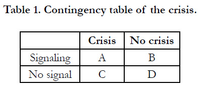

Table 1. Contingency table of the crisis.
However each indicator has different contribution in predicting crisis. In order to consider all the information and the different contribution among the variables at the same time, [55] proposed four methods to assemble the information. Since there is no big difference among these four methods, two methods are introduced here as the benchmarks. First method records the number of indicators signalizing. The more the number of indicators signalizing the more likely the crisis is to occur. Let 1t I represent the index of method one at time t. Sj =1 t represents indicator j is signalizing at time t, and Sj = 0 t otherwise 1t I . is calculated as follows.
where j represents the number of indicators. After this, is viewed as another indicator. The threshold value for this indicator is found in the same way as the other indicators do.
Since method one does not consider the different contribution of each indicator, method two is trying to modify method one by multiplying each j t S with the reciprocal of ω. The index of method two, 2t I , is calculated as follows.
where ωj is the value of of indicator j. Similarly the threshold value of this index is found in the same way as the other indicators do.
Logistic Regression Model
Since the dependent variable, currency crisis, is a binary variable, the logistic regression model is therefore adopted (Baltagi,1995). Let Y = 1 it represent country i has a crisis at time t, and Y = 0 it otherwise. Let it P indicate the probability of country i to have a crisis at time t, then,
E Y = × P + × − P = P ---- (3)
which can be expanded by including n explanatory variables and can be written as the following equation.
where * it y are the actual dependent variable which cannot be observed, is the vector consisting of n explanatory variables, is the vector consisting of n unknown coefficients, is the error term. Then the log-likelihood function can be written as follows.
where is the number of periods, N is the number of countries. The parameters can be obtained through the maximum likelihood method. However, since the data set contains the cross sectional and longitudinal data, it is worthwhile to consider the panel logit to consider both the cross sectional and time series effects simultaneously.
The panel logit with fixed effect model is also named least squares dummy variable model (LSDV), allowing the difference existing in the cross sectional part but no difference for the time series part. In other words, the intercept of the regression model for each country is different and is fixed, showing the difference coming from the different characteristics of each country. The equation can be written as follows.
i=1,2,....I, j=1,2,...J, t=1,2.... T ---- (7)
where i represents the i-th country, j represents the j-th variable, t represents the number of periods, Di is the dummy variable, αiDi represent the specific characteristics of country I, Xijt is the value of the j-th variable of country I at time t, and is the error term of country i at time t.
Panel logit with random effect is also named as error components model, (ECM). This model assumes that the difference among the countries are random, which effects can be described in the error term. The equation can be written as follows.
where i I i i , 1,2, , 0 0 = + = ε β β , i ε is a random variable, and E( i ε ) = 0, var ( i ε ) = 2ε σ . Replace i i β = β +ε 0 0 into equation (7), we could obtain the following result:
in other words, the error term now contains two parts, i ε and it μ . i ε represents the error term of cross sectional part, it μ and represents the error term of the time series part. The general assumptions for the ECM model are as follows (Gujarati, 2003).
Neuro Fuzzy Logic
Basically fuzzy logic is dealing with the extent an object belongs to a fuzzy set. Usually ( ) A μ X is used to describe the extent object x belongs to fuzzy set A. The difference between fuzzy logic and the traditional expert system is that the rules in fuzzy logic are described through the use of linguistic variables instead of the numerical variables. And the linguistic variables are described by several terms. For example, a simple fuzzy logic rule can be stated as follows.
IF export is low and reserve is medium, then currency crisis is high…… [15] where export, reserve, and currency crisis are called linguistic variables; low, medium, and high are the so called terms. Each term has a corresponding membership function. A fuzzy logic model is constructed by a set of “IF-THEN” rules as equation [15] to describe the relationship among the input and output variables. The process to construct a fuzzy logic model generally consists of three main steps, fuzzification, inference, and defuzzification, which are described briefly as follows.
Fuzzification Procedure: The first step in constructing a fuzzy logic is to clearly define the linguistic variables which stated in the “if-then” rules. A linguistic variable can be described by several terms. For example, we can use three terms, high, medium, and low to describe export and reserve. Each term has a corresponding membership function as shown in Figure 1a and 1b. There are four commonly used membership functions, Z, Λ, Π, and S type (91)° Since there is no rule available to decide which type to choose, and the preliminary experiment shows that there is no significant difference for these four different membership functions, we choose the most commonly used one, Λ type membership function.
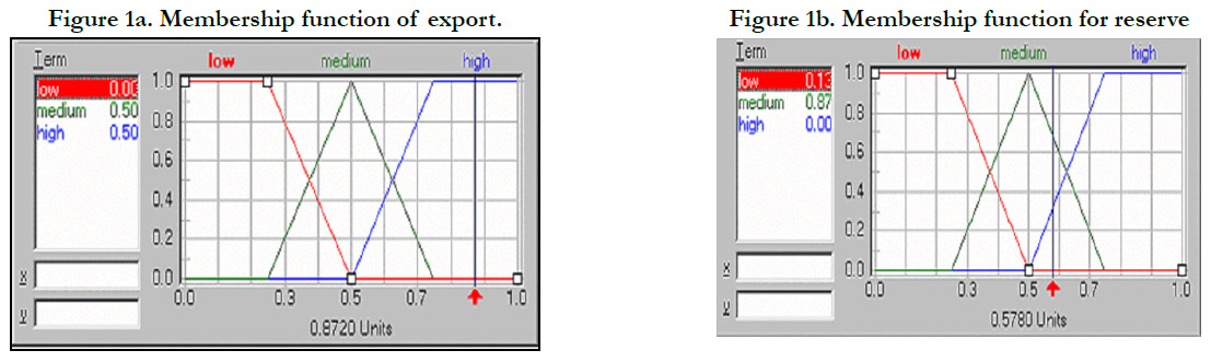
Figure 1a. Membership function of export.
Figure 1b. Membership function for reserve.
Assume there is a country with export and reserve equal to 0.872 and 0.578, respectively. The values for each term can be obtained from figure 1a and 1b as follow.
Export: μlow(0.872) = 0, μmedium (0.872) = 0.5, μhigh(0.872) = 0.5 Reserve: μlow(0.578) = 0.13, μmedium (0.578) = 0.87, μhigh (0.578)=0.00 The above process is what we call fuzzification. Since a linguistic variable can be described by several terms, this method has broken the binary logic constraint.
Inferential Steps: The knowledge base of fuzzy logic is constructed by a series of "If–Then" rules. Each rule consists of two parts, the “if ” part and the “then” part. The "If ” part measures the extent how the condition is satisfied and the “then” part describes how the model responds the input. Therefore, each inference consists of two calculations. The extent of the validity for the then part depends on the extent how the “if ” part is satisfied. According to Thole (1979), the extent how the “if ” part is satisfied is determined as the minimum value of the membership functions in the “if ” part. In other words, min{ , } A B A B μ μ μ ∩ = . Take the above rule for example. Since μhigh(0.872) = 0.5, and μmedium(0.578) = 0.87, the validity of the “if ” part is min{0.8720, 0.5780}=0.5780. Therefore, the output for this rule is currency crisis is low with validity equal to 0.578.
Defuzzification Procedure: After the fuzzification and the inference steps, a result as equation [15], the currency crisis is low with validity equal to 0.578, will be obtained from each rule. Assume that the similar results from the other rules are currency crisis is medium with validity equal to 0.23 and currency crisis is high with validity equal to 0.97. The process to transform these linguistic results into a numerical value is called defuzzification. Usually it entails two steps. First, find out the proxy value for each term. Second, combine these proxy values. Usually the proxy value is determined as the value with the maximum membership function value. Then calculate the weighted value of the proxy value of each term with its membership function value as its weight. For example, if the proxy value for each term is {0.2,0.5,0.7}, then the weighted average is 0.5780* 0.2 + 0.2300*0.5 + 0.9700*0.7 = 0.8236°In other words the probability for currency crisis is 0.8236. This commonly used method is called gravity method (91)°.
The process is what we called the inference mechanism of fuzzy expert system. The problem is that the influence of each rule should be different. The way to improve this is to assign the weight (DOS, degree of support) to each rule, representing the relative importance of each rule compared to the other rules. Then the calculation for the “then” part should be modified as the validity of the “if ” part multiplied by the corresponding weight. However, how can the correct knowledge base be obtained? How to decide the weight for each rule? Among all the possible alternatives, the learning ability of neural network can be used to solve this problem. Therefore, the hybrid of neural network and fuzzy logic can be a good possibility for this problem, which is what we called neuro fuzzy.
Algorithmically, the neuro fuzzy model uses the learning ability of neural network to find the parameters in the fuzzy logic system. In this paper, we adopt the fuzzy associate memory model proposed by Kosko (1992) to implementing the learning process. Each rule is seen as the neuron in the neural networkand the weight of each rule is updated by using back propagation. The knowledge base is obtained when the training stopping criteria is satisfied. Due to its simplicity and learning ability, this method has been applied a lot to many fields (Stoeva, 1992).
The neuro fuzzy model building process is described as follows. Step 1.Divide the data set into in-sample and out-of-sample.
Step 2.Construct the complete knowledge base and set all the weights (DOS)associated with each rule equal to 0 as the initial solution.
Step 3. Use the learning ability of neural network to update the weights. If the relationship described in a rule really exists in the data set, the weight of this rule will be strengthened, otherwise the weight will remain 0. The training process stops when the stopping criterion is satisfied. All the rules with weight value less than a predetermined threshold value will be eliminated, the remaining rules are what we obtain to describe the relationship among the variables existing in the data set.
Step 4. Use the out-of-sample data set to validate the obtained model. If the out-of-sample can be predicted accurately, the model building process stops. Otherwise, repeat step 3 and step 4.
Methodology
Data Set
The data set mainly comes from the work of Kaminsky and Reinhart(
1999), including 20 countries ranging from 1970 June to 1998
June. Some missing values are filled in by referencing to other data
base. It is divided into two parts, in-sample and out-of-sample
data sets. In-sample data set goes from 1970 through 1995, used
for model building. Out-of-sample data goes from 1996 through
1998, used for model validation.
Definition of Crisis
According to Eichengreen, Rose, and Wyplosz(1996), currency
crisis can be measured through the EMP, which is calculated as
follow.
where (% ) i,t Δe is the deflation rate of nominal exchange rate of
country i at time t,% ( ) i,t USA,t Δ i − i is the difference of interest rate
between country i and America, is the change rate of reserve,
α ,β , and γ are the weights to adjust the variance to be equal among
these three parts. A currency crisis can be defined as follows.
where EMPi ,t
μ and EMPi ,t
σ represents the mean and variance of
EMP respectively. This definition is proposed by Sachs, Tornell,
and Velasco (1996) first, and used latter by many researches. Goldstein,
Kaminsky, and Reinhart(2000) modified this formula as follows.
where Δe / e is the change rate of exchange rate, ΔR / R is the
change rate of e σ , is the standard deviation of Δe / e , R σ is the
standard deviation of ΔR / R . The reason to remove the interest
rate change is that some countries adopt the interest rate control
which makes this variable have no significant explanation for
the currency crisis. The function of e R σ σ is similar to that of
α ,β , and γ to adjust the variance of each part equal. This research
will follow the definition of [47] to define a currency crisis occurs
when the EMP is greater than the average at least 3 standard deviations,
otherwise no currency crisis occurs.
The Selection of Indicators
Among the 15 indicators obtained in Kaminsky and Reinhart(
1996), we choose 13 indicators due to the availability of the
data set. They are M2 multiplier, Domestic Credit/GDP、 real
interest rate、Lending-deposit rate ratio、M2/reserves、Bank
Deposits、export、Terms-of-Trade、real exchange rate、Impo
rts、Reserves、output、and Stock Prices. The sources of these
data are listed in Appendix 1.
Performance Criteria
To compare the performance among the models, we use the accuracy rate and noise to signal ratio as the criteria. The accuracy
rate is defined as the ratio of the number of the correct prediction
divided by the total number of predictions. The higher the
accuracy rate the better the model. Similarly the smaller the noise
to signal ratio the better the model is.
Empirical Results and Discussion
Results of the signal approach
The results of the signal approach for the variable sare shown in
table 1. The second column is the threshold value for each variable.
The third column is the accuracy rate. The fourth column is
the noise to signal ratio. The fifth column is the rank of the variables
sorted according to the noise to signal ratio, from small to
large. Besides, we put the empirical results from KLR(1996) at the
right hand side for comparison. Basically the order of the rank is
similar except for some variables. The difference may come from
the data modification every two year, the ways data are transformed,
and the ways to deal with missing values [38].
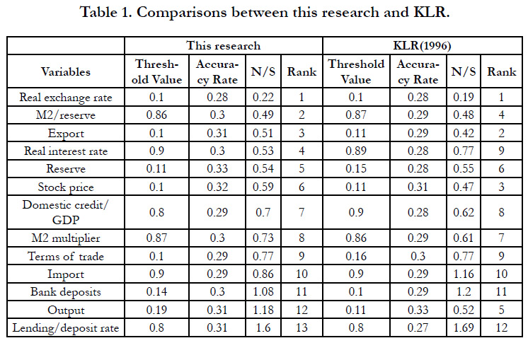
Table 1. Comparisons between this research and KLR.
Comparison between the logit and panel logit
The panel logit results are shown in table 2. All the coefficients are statistically not significant for both random effect and fixed effect models except for the constant term of random effect model. In addition to the panel logits, we construct the logit for each one of the four Asian countries. The empirical results are shown in Table 3. It can be seen that the significant coefficients are different for each countries, implying the inappropriateness of the panel logits. The comparisons among these three models are shown in Table 4. Although the accuracy rate of the logit is worse than that of the panel logits for the in-sample data set, it is the opposite result for the out-of-sample data set.
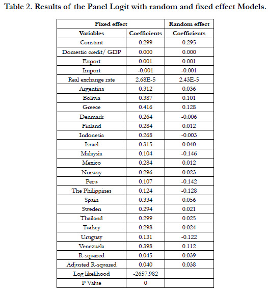
Table 2. Results of the Panel Logit with random and fixed effect Models.
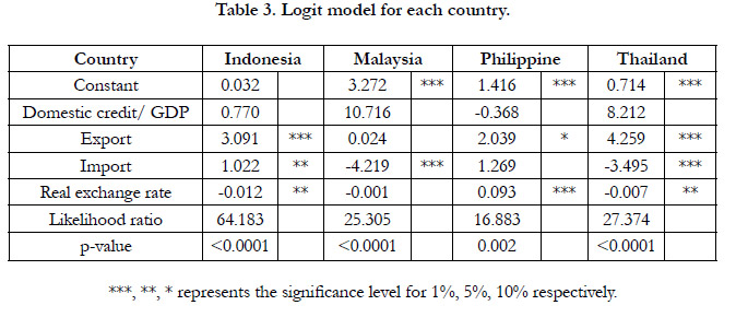
Table 3. Logit model for each country.
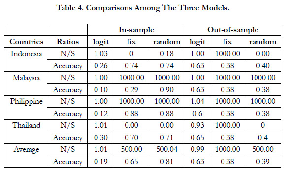
Table 4. Comparisons Among The Three Models.
Since the logit model seems more consistent in terms of both noise to signal ratio and accuracy rate than the panel logits, we use it as the benchmark for the further comparison.
Neuro Fuzzy model
To make the comparison fair, we include the same four variables shown in the logit model into the neuro fuzzy model as input variables. BOP is the output variable representing the probability for a currency crisis to occur. If the probability is greater than a threshold value, it is considered as signalling a warning that a currency crisis is about to happen. Otherwise, there is no currency crisis.
This research describes these four independent variables by using three terms, low, medium, and high, and describes the dependent variable BOP by using five terms, very low, low, medium, high, and very high. Overall this model consists of four input variables, one output variables, and one knowledge base.
As alluded to before, the neuro fuzzy modeling approach(from here on called simply neuro fuzzy) is a fuzzy logic system with the learning ability of neural network to modify its parameters, including the parameters of the membership function and the relative importance of each rule. There are different ways to combine these two techniques (Buckley and Hayashi, 1994; Nauck and Kruse, 1997; Lin and Lee, 1996). These methods turn out to be not so different from one another in practice. This paper adopts the FAM (fuzzy associative memory; FAM) proposed by Kosko (1992). Each rule is viewed as a neuron, the weight of each rule is represented as the weight of each edge in the neural network. For each data point there is a predicted value generated by the system associated with a realized value. The training process will stop until the error between the predicted value and realized value is less than a certain threshold value.
The general neural network model gives the output as a nonlinear function of the data inputs with the specification of the transfer functions in accordance with lowering the errors. Thus the transfer functions connect the hidden node and output node, respectively. The most popular choice for the transfer function specification is the sigmoid function.
In practice matrices of linking weights from input to hidden layer and from hidden to output layer, respectively are found experimentally. The comparisons among the models.
Let SA1 represent the signal approach method one, SA2 the signal approach method two, NF the neuro fuzzy model, and LG the logit model. Due to the availability of the data set, we use the outof- sample data of Indonesia, Malaysia, Philippine, and Thailand for testing. The empirical results are shown in the following two parts, in-sample data set and out-of-sample data set. Forecasting performance for in-sample data: Table 5 shows the forecasting performance of these four models based on the in-sample data set. It can be seen that NF has the lowest noise to signal (n/s) ratio among these models for each country in addition to the lowest average ratio.
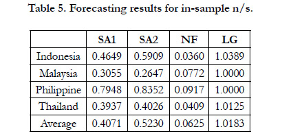
Table 5. Forecasting results for in-sample n/s.
Table 6 shows the accuracy rate of each model for each country. It can also be seen that NF has the highest accuracy rate among the models for each country in addition to the highest average accuracy rate.
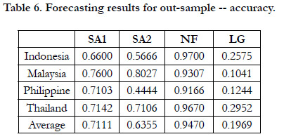
Table 6. Forecasting results for out-sample -- accuracy.
In addition to the noise to signal ratio and the accuracy rate of each model, we also show the signal given by each model during the crisis period and during the tranquil period. The grey area in Figure 3 represents the crisis periods when the model must give a signal to indicate the crisis. We use 1 to represent a signal and 0 to represent non-signal. In other words, during the grey area, if there is a signal, it is a correct signal. If the signal happens outside the grey area, it is a false alarm. Figure 2, 3, 4, and 5 shows the signals given by each model for Indonesia, Malaysia, Philippine, and Thailand respectively.
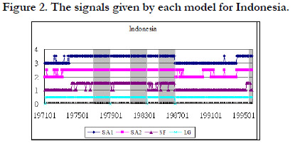
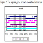
Figure 2. The signals given by each model for Indonesia.
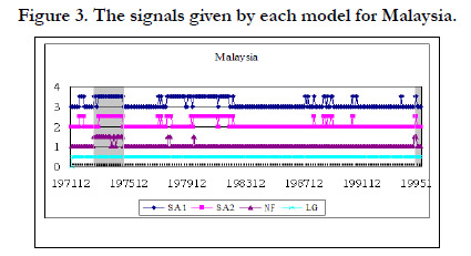
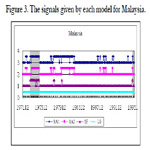
Figure 3. The signals given by each model for Malaysia.
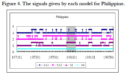
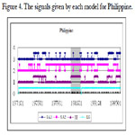
Figure 4. The signals given by each model for Philippine.
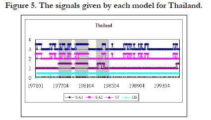
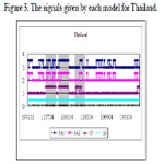
Figure 5. The signals given by each model for Thailand.
Figure 3 shows that almost each model gives a signal during the crisis periods for Indonesia. In other words, each model can effectively signal the crisis. However, they also have many false alarms during the normal periods except NF. LG almost gives a signal all the time. Therefore, NF has the lowest noise to signal ratio and the largest accuracy rate among these models. The similar results are shown in figure 3, 4, and 5 for Malaysia, Philippine, and Thailand.
Forecasting performance for out-of-sample data: Table 7 shows the noise to signal ratio of each model for each country. It can be seen that NF has the lowest average ratio among these four methods in addition to the lowest ratio for each country. Table 8 shows the accuracy rate of each model for each country. It can also be seen that NF has the highest average accuracy rate in addition to the highest accuracy rate for each country.
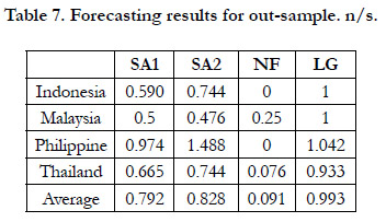
Table 7. Forecasting results for out-sample. n/s.
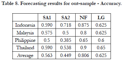
Table 8. Forecasting results for out-sample - Accuracy.
Figure 5 to figure 8 shows the signals given by each model for each country. The results are similar to the training data set.
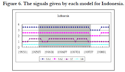
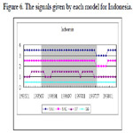
Figure 6. The signals given by each model for Indonesia.
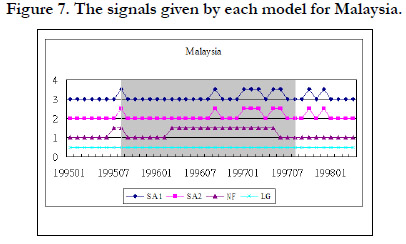
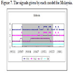
Figure 7. The signals given by each model for Malaysia.
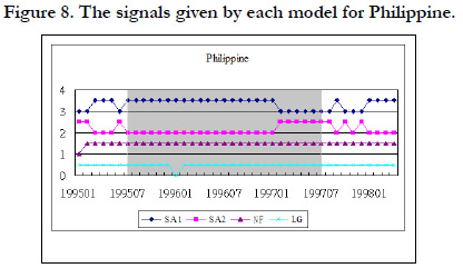
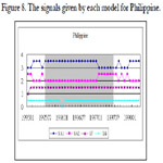
Figure 8. The signals given by each model for Philippine.
Conclusion
It will not be an overstatement to say that in the 21st century
the related fields of Artificial Intelligence(AI) and Machine
Learning(ML) have made rapid progress. So much so that their
algorithmic approaches have become common outside of economics.
We have tried to show in this paper through formal AI
and ML modeling in an important area of international financial
economics that it is possible to demonstrate that certain AI and
ML type of modeling has great relevance for difficult areas of
international financial economics and complex financial systems
analysis. We follow scholars such as A they who have pointed
out that AI and ML have great relevance for causal analysis of
economic problems along with standard econometrics causality
exploration techniques. We have shown through our formal and
empirical demonstrations how we can illustrate at least one strand
of this general argument for complementarity of econometrics and AI-based ML by considering machine learning type of AI
in a neural network and fuzzy set theoretic formal setting. Our
hybrid model appears to predict comparatively better the currency
crises by using neuro fuzzy approach to ML, which combines the
learning ability of neural network and the inference mechanism
of fuzzy logic.
Since currency crises have been important and puzzling areas of
international finance from at least the last decade of the 20th century
throughout the 21st century so far. In order to avoid the
devastating damage caused by such crises often leading to broader
financial and economic crises, we need an effective early warning system. This paper shows how to make a start on this by trying
to construct an early warning system through the AI-based ML
using the neuro fuzzy nonlinear modeling technique. We compare
its forecasting performance with those of signal approach and
logit models. The empirical results show that our ML-based neuro
fuzzy model can providerealtively a high accuracy rate of 80.62%
for the out of sample data set. Besides, the knowledge base provides
a more detailed relationship among the variables, showing
how to make further progress towards averting or at least mitigating
the worst effects of the crisis through the construction of a
relatively more effective early warning system. The 3-dimensional
graphics can also show a more clear relationship depicting the
interaction effects between the key variables. These relationships
can also be the basis for theoretical modification for further research
for modeling inductive learning.
References
-
[1]. Abadie A, Cattaneo MD. Econometric methods for program evaluation. Annual
Review of Economics. 2018 Aug 2;10:465-503.
[2]. Abadie A, Imbens GW. Bias-corrected matching estimators for average treatment effects. Journal of Business & Economic Statistics. 2011 Jan 1;29(1):1- 1.
[3]. Abadie A, Diamond A, Hainmueller J. Synthetic control methods for comparative case studies: Estimating the effect of California’s tobacco control program. Journal of the American statistical Association. 2010 Jun 1;105(490):493-505.
[4]. Abadie A, Diamond A, Hainmueller J. Comparative politics and the synthetic control method. American Journal of Political Science. 2015 Feb;59(2):495- 510.
[5]. Angrist, Joshua D and J¨orn-Steffen Pischke. Mostly harmless econometrics: An empiricist’s companion. Princeton University Press, 2008.
[6]. Arjovsky M, Bottou L. Towards principled methods for training generative adversarial networks. arXiv preprint arXiv:1701.04862. 2017 Jan 17.
[7]. Arora S, Y Li, Y Liang, T Ma. RAND-WALK: A latent variable model approach to word embeddings. Transactions of the Association for Computational Linguistics, 4, 2016.
[8]. Athey S. Beyond prediction: Using big data for policy problems. Science. 2017 Feb 3;355(6324):483-5.
[9]. Susan Athey. The impact of machine learning on economics. The Economics of Artificial Intelligence, 2018.
[10]. Athey S, Imbens G. Recursive partitioning for heterogeneous causal effects. Proceedings of the National Academy of Sciences. 2016 Jul 5;113(27):7353- 60.
[11]. Athey S, Imbens GW. The econometrics of randomized experiments. In- Handbook of economic field experiments 2017 Jan 1; 1: 73-140.
[12]. Athey S, Imbens GW. The state of applied econometrics: Causality and policy evaluation. Journal of Economic Perspectives. 2017 May;31(2):3-2.
[13]. Athey S, Stefan Wager. Efficient policy estimation. arXiv preprint arXiv: 1702.02896, 2017.
[14]. Athey S, Imbens GW, Wager S. Efficient inference of average treatment effects in high dimensions via approximate residual balancing. 2016 Apr.
[15]. Athey S, Tibshirani J, Wager S. Generalized random forests. The Annals of Statistics. 2019 Apr;47(2):1148-78.
[16]. Athey S, Bayati M, Doudchenko N, Imbens G, Khosravi K. Matrix completion methods for causal panel data models. Journal of the American Statistical Association. 2021 Apr 21:1-5.
[17]. Donnelly R, Ruiz FR, Blei D, Athey S. Counterfactual inference for consumer choice across many product categories. arXiv preprint arXiv:1906.02635. 2019 Jun 6.
[18]. Athey S, Mobius M, Pal J. The impact of aggregators on internet news consumption. National Bureau of Economic Research; 2021 May 3.
[19]. Athey S, Julie Tibshirani, Stefan Wager. Generalized random forests. arXiv preprint arXiv:1610.01271, 2017.
[20]. Athey S, Bayati M, Imbens G, Qu Z. Ensemble methods for causal effects in panel data settings. InAEA Papers and Proceedings 2019 May 109; 65-70. [21]. Bamler R, Mandt S. Dynamic word embeddings via skip-gram filtering. stat. 2017 Feb;1050:27.
[22]. Barkan O. Bayesian neural word embedding. InThirty-First AAAI Conference on Artificial Intelligence 2017 Feb 12.
[23]. Agenor PR, Bhandari JS, Flood RP. Speculative attacks and models of balance of payments crises. Staff Papers. 1992 Jun;39(2):357-94.
[24]. Berg A, Pattillo C. Are currency crises predictable? A test. IMF Staff papers. 1999 Jun;46(2):107-38.
[25]. Blanco H, Garber PM. Recurrent devaluation and speculative attacks on the Mexican peso. Journal of political economy. 1986 Feb 1;94(1):148-66.
[26]. Calvo G, E Mendoza. “Reflections on Mexico’s Balance-of-Payments Crisis: A Chronicle of Death Foretold.” unpublished; College Park: University of Maryland, 1995.
[27]. Chowdhry B, Goyal A. Understanding the financial crisis in Asia. Pacific- Basin Finance Journal. 2000 May 1;8(2):135-52.
[28]. Cole H, Kehoe T. A self-fulfilling model of Mexico’s 1994-5 debt crisis. Federal Reserve Bank of Minneapolis. Staff Report 210; 1996.
[29]. Collins SM. The timing of exchange rate adjustment in developing countries. April, Georgetown University and Brookings Institution. 1995.
[30]. Connolly M. Exchange rates, real economic activity and the balance of payments: evidence from the 1960s. Recent Issues in the Theory of the Flexible Exchange Rates. 1983:129-43.
[31]. Cumby RE, Van Wijnbergen S. Financial policy and speculative runs with a crawling peg: Argentina 1979–1981. Journal of international Economics. 1989 Aug 1;27(1-2):111-27.
[32]. Diebold FX, GD. Rudebusch. “Scoring the Leading Indicators.” Journal of Business. 1989; 62 (3):369-391.
[33]. Domingos P. A few useful things to know about machine learning. Communications of the ACM. 2012 Oct 1;55(10):78-87.
[34]. Hasperué W. The master algorithm: how the quest for the ultimate learning machine will remake our world. Journal of Computer Science and Technology. 2015 Nov 1;15(02):157-8.
[35]. Dooley MP.“A Model of Crises in Emerging Markets.” NBER Working Paper, 1997 December (6300) :1-33.
[36]. Dornbusch R, Goldfajn I, Valdés RO, Edwards S, Bruno M. Currency crises and collapses. Brookings papers on economic activity. 1995 Jan 1;1995(2):219-93.
[37]. Dornbusch R, Cline WR. Brazil's incomplete stabilization and reform. Brookings Papers on Economic Activity. 1997 Jan 1;1997(1):367-404.
[38]. Edison HJ. “Do Indicators of Financial Crises Work? An Evaluation of An Early Warning System.” International Finance Discussion Papers. 2000.
[39]. Eichengreen B, Rose AK, Wyplosz C. Exchange market mayhem: the antecedents and aftermath of speculative attacks. Economic policy. 1995 Oct 1;10(21):249-312.
[40]. Eichengreen B, AK Rose, C Wyplosz. “Contagious Currency Crises” Centre for Economic Policy Research(London) Discussion Paper, No. 1453( August). 1996.
[41]. Eichengreen B, Rose AK, Wyplosz C. Exchange market mayhem: the antecedents and aftermath of speculative attacks. Economic policy. 1995 Oct 1;10(21):249-312.
[42]. Flood R, N Marion.“Perspecitives on the Recent Currency Crisis Literature.” NBER Working Paper No. 6380 (Cambridge, Massachusetts: National Bureau of Economic Research). 1998.
[43]. Frankel JA, Rose AK. Currency crashes in emerging markets: An empirical treatment. Journal of international Economics. 1996 Nov 1;41(3-4):351-66. [44]. Gerlach S, F Smets.“Contagious Speculative Attacks.” CEPR Discussion Paper, No. 1055(November). 1994.
[45]. Goldfajn I, RO Valdes.“Balance-of-Payments Crises and Capital Flows: The Role of Liquidity.” Mimeo, Massachusetts Institute of Technology. 1995. [46]. Goldstein M. Presumptive indicators/Early warning signals of vulnerability to financial crises in emerging market economies. Unpublished paper. 1996 Jan.
[47]. Goldstein M, Kaminsky GL, Reinhart CM. Assessing financial vulnerability: an early warning system for emerging markets. Peterson Institute; 2000. [48]. Gylfason T, Schmid M. Does devaluation cause stagflation?. Canadian Journal of Economics. 1983 Nov 1:641-54.
[49]. Gylfason T, O Risager. "Does Devaluation Improve the CruuentAccount?" European Economic Review, 1984: 37-64.
[50]. International Monetary Fund (IMF). World Economic Outlook (May) 1998. [51]. Trevor Hastie, Robert Tibshirani, Jerome Friedman. The Elements of Statistical Learning. New York: Springer, 2009.
[52]. Trevor Hastie, Robert Tibshirani, Martin Wainwright. Statistical Learning with Sparsity: The Lasso and Generalizations. CRC Press, 2015.
[53]. Trevor Hastie, Robert Tibshirani, Ryan J Tibshirani. Extended comparisons of best subset selection, forward stepwise selection, and the lasso. arXiv preprint arXiv:1707.08692, 2017.
[54]. Hinton, Geoffrey. “Learning distributed representations of concepts”. Proceedings of the Eighth Annual Conference of the Cognitive Science Society, Amherst, Mass. Reprinted in Morris, R. G. M. editor, Parallel Distributed Processing: Implications for Psychology and Neurobiology, Oxford University Press, Oxford, UK. 1986.
[55]. Kaminsky GL, Reinhart CM. The twin crises: the causes of banking and balance-of-payments problems. American economic review. 1999 Jun;89(3):473-500.
[56]. Kaminsky GL, Leiderman L.“High Real Interest Rates in the Aftermath of Disinflation Credit Crunch or Credibility Crisis?” forthcoming in Journal of Development Economics. 1998.
[57]. Kaminsky G, Lizondo S, Reinhart CM. Leading indicators of currency crises. Staff Papers. 1998 Mar;45(1):1-48.
[58]. Kennedy, Peter: A Guide to Econometrics, 4th ed., MIT Press, Cambridge, Mass., 1998.
[59]. Khan, Haider A. forthcoming. Governing a Complex Global Financial System in the Age of Global Instabilities and BRICS : Promoting Global Financial Stability and Growth with Equity, in PB Anand, Flavio Comim, Shailaja Fennell, John Weiss eds. Oxford Handbook of BRICS and Emerging Economies, Oxford University Press, 2019.
[60]. Khan HA. Causal Depth and Counterfactuals for Scientific Explanation and an Ethically Efficacious Economics: How can economics and the social sciences help make policies for advancing the common good?, JKSIS Working Paper. 2019b
[61]. Khan HA. On paradigms, theories and models. Problemas del Desarrollo. 2003 Jul 1;34(134):149-55.
[62]. Khan HA . Global Markets and Financial Crisis: Towards a Theory for the 21st Century, Basingstoke, UK: Macmillan/Palgrave. 2004
[63]. Khan HA. “Managing global risks and creating prosperity : the role of the IMF and regional financial architectures” in Junji Nakagawa, ed. Managing Development: Globalization, Economic Restructuring and SocialPolicy, Routledge. 2006: 17-41.
[64]. Khan H. Causal Depth contra Humean Empiricism: Aspects of a Scientific Realist Approach to Explanation. 2008.
[65]. Khan HA. Analyzing the impact on financial crisis on developing countries. Report submitted to the UNDP, NYC. 2011.
[66]. Khan HA . “Development Strategies: Lessons from South Korea, Thailand, Malaysia and Viet Nam”, in Augustin Fosu ed. Lessons from Successful Development Strategies, Oxford:Oxford University Press. 2013a
[67]. Haider KH. BASEL III, BANK FOR INTERNATIONAL SETTLEMENTS AND. Journal of Advanced Studies in Finance (JASF). 2013;4(08):121-44. [68]. Klein, MW, N Marion. “Explaining the Duration of Exchange-Rate Pegs.” NBER Working 4651: 1994.
[69]. Krugman P. A model of balance-of-payments crises. Journal of money, credit and banking. 1979 Aug 1;11(3):311-25.
[70]. Krugman P. Are currency crises self-fulfilling?. NBER Macroeconomics annual. 1996 Jan 1;11:345-78.
[71]. Mc Kinnon, RI, H Pill.“Credible Liberalizations and International Capital Flows: The ‘Overborrowing Syndrome’.” in Takatoshi Ito and Anne O. Krueger, eds., Financial Deregulation and integration in East Asia. Chicago: University of Chicago Press, 7-42: 1996.
[72]. Khan Haider A. A New Approach to Modeling Early Warning Systems for Financial Crises. Journal of International Money and Finance. 2008:1098-121.
[73]. Lin CS, Khan HA, Huang CC. Can the neuro fuzzy model predict stock indexes better than its rivals?. Discussion Papers of University of Tokyo CIRJEF- 165. 2002 Aug.
[74]. Milesi-Ferretti GM, A Razin.“Current Account Sustainability.” Priceton Studies in International Finance, No. 81(Princeton, New Jersey Princeton University, Department of Economics, International Finance Section, October). 1996.
[75]. Milesi-Ferretti GM, Razin A. Determinants and Consequences of Current Account Reversals and Currency Crises. International Monetary Fund, Washington, DC. 1998 Feb 6-7.
[76]. Mishkin FS.“Understanding Financial Crises: A Developing Country Perspective.” in Michael Bruno and Boris Pleskovic, eds., Annual World Bank conference on development economics. Washington DC: World Bank, pp. 1996: 29-62.
[77]. Moreno R. “Macroeconomic Behavior During Periods of Speculative Pressure or RealignmentEvidence from Pacific Basin Countries.” Economic Review, Federal Reserve Bank of San Francisco, No. 1995; (3): 3-16. [78]. Obstfeld M.“Balance-of-payments crises and devaluation.” Journal of Money, Credit and Banking. 1984: 208-219.
[79]. Obstfeld M.“The Logic of Currency Crises.” NBER Working Paper, No. 4640. 1994.
[80]. Obstfeld M. Models of currency crises with self-fulfilling features. European economic review. 1996 Apr 1;40(3-5):1037-47.
[81]. Ötker MI, Pazarbasioglu C. Exchange market pressures and speculative capital flows in selected European countries. International Monetary Fund; 1994 Feb 1.n
[82]. Otker I, C Pazarbasioglu. 1996.“Speculative Attacks and Currency Crises: The Mexican Experience.” Open Economics Review, 1996; 7 (1): 535-552.
[83]. Ozkan FG, Sutherland A. Policy measures to avoid a currency crisis. The Economic Journal. 1995 Mar 1;105(429):510-9.
[84]. Peltonen T. Are currency crises predictable? An application of panel estimation methods and artificial neural networks. Department of Economics, European University Institute, Florence. 2002.
[85]. Rumelhart DE, Hinton GE, Williams RJ. Learning representations by backpropagating errors. nature. 1986 Oct;323(6088):533-6.
[86]. James L. McClelland and PDP Research Group (1987). Parallel Distributed Processing: Explorations in the Microstructure of Cognition, Cambridge, Ma.: The MIT Press.s
[87]. Sachs JD, Tornell A, Velasco A. Financial crises in emerging markets: the lessons from 1995: 147-215.
[88]. Sachs J. What investors should learn from the crisis that has forced Thailand to seek an IMF loan. Financial Times. 1997.
[89]. Edwards S. “Are Devaluations Contractionary?” The Review of Economics and Statistics, 1986: 501-508.
[90]. Stoker J.“Intermediation and the Business Cycle Under specie Standard: The Role of the Gold Standard in English Financial Crises, 1790-1850.” Mineo, University of Chicago. 1994.
[91]. Von Altrock C. Fuzzy Logic & Neuro Fuzzy Applications in Business & Finance. Prentice Hall PTR, Upper Saddle River, NJ. 1996.
[92]. Velasco A. Financial crises and balance of payments crises: a simple model of the southern cone experience. Journal of development Economics. 1987 Oct 1;27(1-2):263-83.